Indices and Confidence Intervals for Statistical Process Control in Python
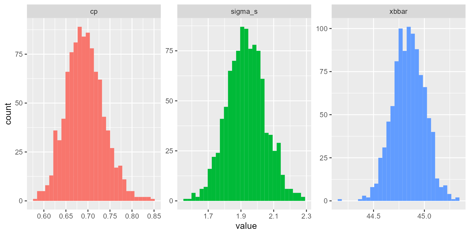
This workshop extends our toolkit developed earlier, discussing Process Capability and Stability Indices, and introducing means to calculate confidence intervals for these indices using Python. We'll calculate Cp, Cpk, Pp, and Ppk, then construct normal-approximation confidence intervals and a simple bootstrap, paralleling the R chapter.
Getting Started
Packages
We'll be using pandas for data manipulation, plotnine for visualization, scipy for statistical functions, and custom functions from the functions_distributions module.
# Remember to install these packages using a terminal, if you haven't already!
!pip install pandas plotnine scipy# Load our packages
import pandas as pd
from plotnine import *
import numpy as np
from scipy import statsCustom Functions
This workshop uses custom functions from the functions_distributions.py module. Download it straight from this site — this is the copy the chapter runs on:
# Download the functions file directly
curl -O https://timothyfraser.com/sigma/data/functions/functions_distributions.py
It also ships in the course code repository, github.com/timothyfraser/sysen, under functions/.
Add the functions directory to your Python path
import sys
import os
# Add the functions directory to Python path
sys.path.append('functions')  # or path to wherever you placed the functions folder
Once you have the functions available, you can import them:
from functions_distributions import *
Our Data
We'll be continuing to analyze our quality control data from a local hot springs inn (onsen) in sunny Kagoshima Prefecture, Japan. Every other month, across a 15-month stretch, you systematically took 20 random samples of hot spring water on each of those 8 sampling months (160 samples in all), and recorded its temperature, pH, and sulfur levels. How might you determine if this onsen is at risk of slipping out of one sector of the market (eg. Extra Hot!) and into another (just normal Hot Springs?).
Let's read in our data from workshops/onsen.csv!
# Let's import our samples of bathwater over time!
water = pd.read_csv('workshops/onsen.csv')
# Take a peek!
print(water.head(3))
print(f"Dataset shape: {water.shape}")
print(f"Columns: {list(water.columns)}")
Our dataset contains:
id: unique identifier for each sample of onsen water.time: categorical variable describing date of sample (month1, month3, ... month15).temp: temperature of the hot spring water in Celsius.ph: pH level of the hot spring water.sulfur: sulfur content in mg per kg of water.
Process Overview
Let's get a visual overview of our temperature data across time to understand the process:
# Create a process overview plot
g = (ggplot(water, aes(x='time', y='temp')) +
     geom_point(alpha=0.6, size=2) +
     geom_hline(yintercept=[42, 50], color=['red', 'red'], linetype='dashed') +
     theme_classic(base_size=14) +
     labs(x='Time (Month)', y='Temperature (°C)',
          title='Hot Spring Temperature Over Time',
          subtitle='Red dashed lines show specification limits (42-50°C)') +
     theme(plot_title=element_text(hjust=0.5),
           plot_subtitle=element_text(hjust=0.5)))

# Save the plot
g.save('images/06_process_overview.png', width=10, height=6, dpi=100)
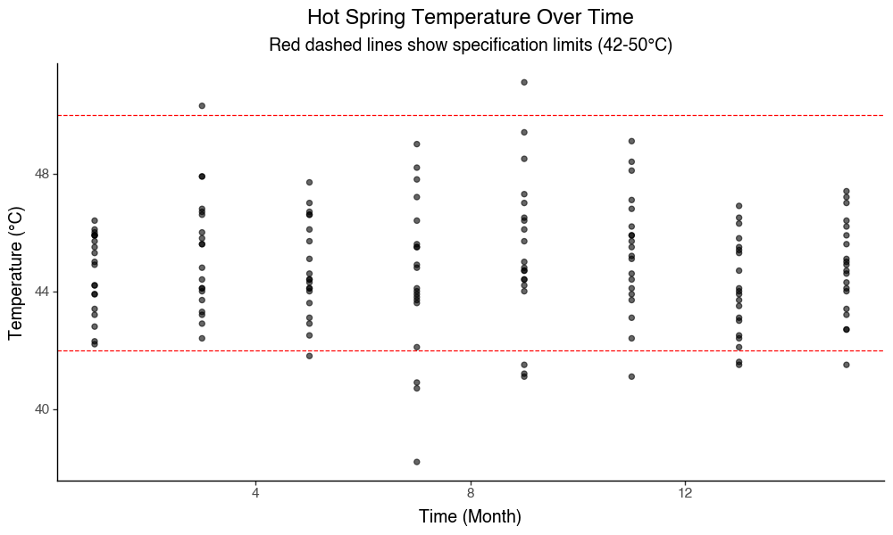
This plot shows our temperature measurements over time, with the specification limits for "Extra Hot Springs" (42-50°C) marked as red dashed lines. We can see the process variation and how it relates to our target specifications.
Process Capability vs. Stability
Definitions
Production processes can be categorized in terms of Capability (does it meet required specifications?) and Stability (is production consistent and predictable?) Both are vital.
- A capable process delivers goods that can actually perform their function, like a 20-foot ladder that is actually 20 feet!
- A stable process delivers products with consistent and predictable traits (regardless of whether those traits are good).
We need to maximize both process capability and stability to make an effective process, be it in manufacturing, health care, local businesses, or social life! Depending on the shape and stability of our data, we should choose one of the 4 statistics to evaluate our data.
Table of Indices
These statistics rely on some combination of (1) the mean \( \mu \), (2) the standard deviation \( \sigma \), and (3) the upper and lower "specification limits"; the specification limits are our expected values \( E_{upper} \) and \( E_{lower} \), as compared to our actual observed values, summarized by \( \mu \) and \( \sigma \).
| Index | Shape | Sided | Stability | Formula | Meaning |
|---|---|---|---|---|---|
| \( C_{p} \) | Centered | 2-sided | Stable | \( \frac{E_{upper} - E_{lower}}{6 \sigma_{short}} \) | How many times wider is the expected range than the observed range, assuming it is stable? |
| \( C_{pk} \) | Uncentered | 1-sided | Stable | \( \frac{\mid E_{limit} - \mu \mid}{3 \sigma_{short}} \) | How many times wider is the expected vs. observed range for the left/right side, assuming it is stable? |
| \( P_{p} \) | Centered | 2-sided | Unstable | \( \frac{E_{upper} - E_{lower}}{6 \sigma_{total}} \) | How many times wider is the expected vs. observed range, stable or not? |
| \( P_{pk} \) | Uncentered | 1-sided | Unstable | \( \frac{\mid E_{limit} - \mu \mid}{3 \sigma_{total}} \) | How many times wider is the expected vs. observed range for the left/right side, stable or not? |
Capability Indices (How could it perform, if stable?): \( C_p \), \( C_{pk} \)
Process Performance Indices (How is it performing, stable or not?): \( P_p \), \( P_{pk} \)
Index Functions
Let's do ourselves a favor and write up some simple functions for these.
def cp(sigma_s, upper, lower):
  """Capability index for centered, stable processes"""
  return abs(upper - lower) / (6*sigma_s)

def pp(sigma_t, upper, lower):
  """Performance index for centered, unstable processes"""
  return abs(upper - lower) / (6*sigma_t)

def cpk(mu, sigma_s, lower=None, upper=None):
  """Capability index for uncentered, stable processes"""
  a = None; b = None
  if lower is not None:
    a = abs(mu - lower) / (3*sigma_s)
  if upper is not None:
    b = abs(upper - mu) / (3*sigma_s)
  if (lower is not None) and (upper is not None):
    return min(a,b)
  return a if upper is None else b

def ppk(mu, sigma_t, lower=None, upper=None):
  """Performance index for uncentered, unstable processes"""
  a = None; b = None
  if lower is not None:
    a = abs(mu - lower) / (3*sigma_t)
  if upper is not None:
    b = abs(upper - mu) / (3*sigma_t)
  if (lower is not None) and (upper is not None):
    return min(a,b)
  return a if upper is None else b
Ingredients
Now we need to calculate the key statistics that feed into our capability indices. We'll calculate both within-subgroup statistics (for capability indices) and total statistics (for performance indices).
stat_s = (water.groupby('time').apply(lambda d: pd.Series({
  'xbar': d['temp'].mean(),
  's': d['temp'].std(),
  'n_w': len(d)
})).reset_index())

stat = pd.DataFrame({
  'xbbar': [stat_s['xbar'].mean()],
  'sigma_s': [(stat_s['s']**2).mean()**0.5],
  'sigma_t': [water['temp'].std()],
  'n': [stat_s['n_w'].sum()],
  'n_w': [stat_s['n_w'].iloc[0]],
  'k': [len(stat_s)]
})
stat
These statistics give us:
- xbbar: The grand mean across all subgroups
- sigma_s: The pooled within-subgroup standard deviation (for capability indices)
- sigma_t: The total process standard deviation (for performance indices)
- n: Total number of observations
- n_w: Number of observations per subgroup
- k: Number of subgroups
Cp and Pp
Now let's calculate the capability and performance indices. We'll use specification limits for "Extra Hot Springs" (42-50°C) as our target range.
limit_lower = 42; limit_upper = 50
estimate_cp = cp(stat['sigma_s'][0], upper=limit_upper, lower=limit_lower)
estimate_pp = pp(stat['sigma_t'][0], upper=limit_upper, lower=limit_lower)
print(f"Cp (capability): {estimate_cp:.3f}")
print(f"Pp (performance): {estimate_pp:.3f}")
Cpk and Ppk
Now let's calculate the uncentered indices that account for process centering:
estimate_cpk = cpk(mu=stat['xbbar'][0], sigma_s=stat['sigma_s'][0], lower=limit_lower, upper=limit_upper)
estimate_ppk = ppk(mu=stat['xbbar'][0], sigma_t=stat['sigma_t'][0], lower=limit_lower, upper=limit_upper)
print(f"Cpk (capability, uncentered): {estimate_cpk:.3f}")
print(f"Ppk (performance, uncentered): {estimate_ppk:.3f}")
Equality
There's an interesting mathematical relationship between these indices:
equality_check = np.isclose(estimate_pp * estimate_cpk, estimate_ppk * estimate_cp)
print(f"Pp × Cpk = Ppk × Cp: {equality_check}")
print(f"Pp × Cpk = {estimate_pp * estimate_cpk:.6f}")
print(f"Ppk × Cp = {estimate_ppk * estimate_cp:.6f}")
Why np.isclose() instead of ==? The identity is exact in algebra, but each index arrives in Python as a rounded binary number, so the two products can differ in the very last digit and == reports False; np.isclose() asks the question we actually mean - are these equal to within floating-point precision?
Let's apply this to some tasty examples! A manufacturer of granola bars is aiming for a weight of 2 ounces (oz), plus or minus 0.05 oz. Suppose the standard deviation of our granola bar machine is 0.02 oz, and the mean weight is 2.01 oz.
What's the process capability index? (I.e. How many times greater is the expected variation than the observed variation?)
cp() function you already wrote: it needs sigma_s plus the upper and lower spec limits (2 ± 0.05). For a one- or two-sided check with cpk(), you'll also need mu, the observed mean.lower = 2 - 0.05 upper = 2 + 0.05 sigma = 0.02 mu = 2.01 # Cp = |2.05 - 1.95| / (6 * 0.02) = 0.8333 print(cp(sigma_s=sigma, upper=upper, lower=lower)) # Cpk = min(2.05 - 2.01, 2.01 - 1.95) / (3 * 0.02) = 0.6667 print(cpk(mu=mu, sigma_s=sigma, lower=lower, upper=upper))
Confidence Intervals (Normal Approximation)
Now let's construct confidence intervals for our capability indices using the normal approximation method. This gives us a range of plausible values for the true population parameters.
Cp Confidence Interval
import math
v_short = stat['k'][0]*(stat['n_w'][0] - 1)
se_cp = estimate_cp * math.sqrt(1 / (2*v_short))
z = 1.959963984540054  # 95% confidence level
ci_cp = (estimate_cp - z*se_cp, estimate_cp + z*se_cp)
print(f"Cp estimate: {estimate_cp:.3f}")
print(f"Standard error: {se_cp:.3f}")
print(f"95% Confidence interval: ({ci_cp[0]:.3f}, {ci_cp[1]:.3f})")
Cpk Confidence Interval
se_cpk = estimate_cpk * math.sqrt(1 / (2*v_short) + 1 / (9*stat['n'][0]*(estimate_cpk**2)))
ci_cpk = (estimate_cpk - z*se_cpk, estimate_cpk + z*se_cpk)
print(f"Cpk estimate: {estimate_cpk:.3f}")
print(f"Standard error: {se_cpk:.3f}")
print(f"95% Confidence interval: ({ci_cpk[0]:.3f}, {ci_cpk[1]:.3f})")
Pp and Ppk Confidence Intervals
v_total = stat['n_w'][0]*stat['k'][0] - 1
se_pp = estimate_pp * math.sqrt(1 / (2*v_total))
ci_pp = (estimate_pp - z*se_pp, estimate_pp + z*se_pp)
print(f"Pp estimate: {estimate_pp:.3f}")
print(f"Standard error: {se_pp:.3f}")
print(f"95% Confidence interval: ({ci_pp[0]:.3f}, {ci_pp[1]:.3f})")

se_ppk = estimate_ppk * math.sqrt(1 / (2*v_total) + 1 / (9*stat['n'][0]*(estimate_ppk**2)))
ci_ppk = (estimate_ppk - z*se_ppk, estimate_ppk + z*se_ppk)
print(f"\nPpk estimate: {estimate_ppk:.3f}")
print(f"Standard error: {se_ppk:.3f}")
print(f"95% Confidence interval: ({ci_ppk[0]:.3f}, {ci_ppk[1]:.3f})")
Visualizing Confidence Intervals
Let's create a visualization to show our Cp estimate with its confidence interval and important benchmark lines:
# Create a DataFrame for plotting
bands_data = pd.DataFrame({
    'index': ['Cp Index'],
    'estimate': [estimate_cp],
    'lower': [ci_cp[0]],
    'upper': [ci_cp[1]]
})

# Create the plot
g = (ggplot(bands_data, aes(x='index', y='estimate', ymin='lower', ymax='upper')) +
     geom_hline(yintercept=[0, 1, 2], color=['grey', 'black', 'grey']) +
     geom_point(size=3) +
     geom_linerange(size=1) +
     theme_classic(base_size=14) +
     coord_flip() +
     labs(y='Index Value', x=None) +
     theme(axis_text_y=element_blank(), axis_ticks_y=element_blank()))

# Save the plot
g.save('images/06_confidence_interval_plot.png', width=8, height=4, dpi=100)
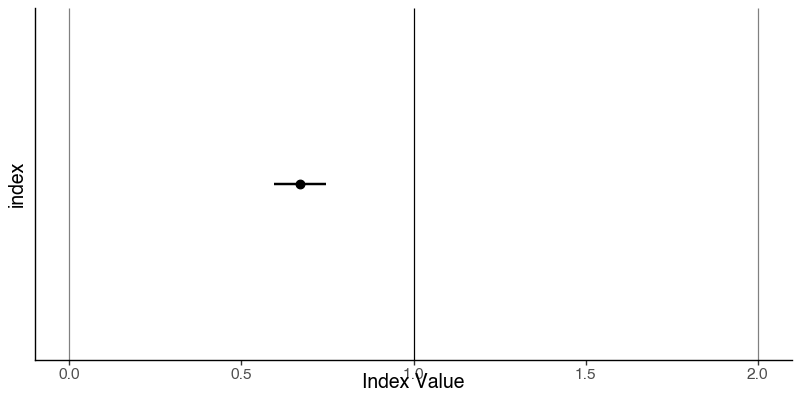
It's not the most exciting plot, but it does show very clearly that the value of \( C_{p} \) and its 95% confidence interval are nowhere even close to 1.0, the key threshold. This means we can say with 95% confidence that the true value of \( C_{p} \) is less than 1.
One-Sided Bounds
Look again at that last sentence: we only asked whether \( C_{p} \) sits below 1. That is a one-directional question, and a two-sided interval spends half of its error on the side we don't care about. Plenty of quality questions only have one side:
- A lower bound is a floor: "we are 95% confident that reliability (or \( C_{pk} \), or mean temperature) is at least ___."
- An upper bound is a ceiling: "we are 95% confident that the defect rate (or failure rate) is at most ___."
For a one-sided bound at confidence level \( 1 - \alpha \), put all of \( \alpha \) in one tail. So you take the quantile at \( 1 - \alpha \) instead of \( 1 - \alpha/2 \):
- Lower bound: \( \hat{\theta} - z_{1-\alpha} \cdot SE \)
- Upper bound: \( \hat{\theta} + z_{1-\alpha} \cdot SE \)
At 95% confidence, \( \alpha = 0.05 \), so a one-sided bound uses stats.norm.ppf(0.95) (about 1.645), where the two-sided interval above used stats.norm.ppf(0.975) (about 1.96). If your statistic follows a t distribution instead (like a mean), swap in stats.t.ppf(1 - alpha, df) the same way.
alpha = 0.05  # 95% confidence
# ALL of alpha goes in one tail: the 95th percentile, not the 97.5th
z_one = stats.norm.ppf(1 - alpha)  # about 1.645
# Report ONE of these - whichever side answers your question
lower_cp = estimate_cp - z_one*se_cp  # a floor: "Cp is at least..."
upper_cp = estimate_cp + z_one*se_cp  # a ceiling: "Cp is at most..."
print(f"z one-sided: {z_one:.3f} vs. two-sided: {z:.3f}")
print(f"95% lower bound for Cp: {lower_cp:.3f}")
print(f"95% upper bound for Cp: {upper_cp:.3f}")

# Same rule with a t quantile: a floor on mean temperature
n_temp = len(water)
se_mean = water['temp'].std() / math.sqrt(n_temp)
t_one = stats.t.ppf(1 - alpha, df=n_temp - 1)
print(f"95% lower bound for mean temp: {water['temp'].mean() - t_one*se_mean:.2f}")
Our 95% upper bound says the true \( C_{p} \) is at most about 0.735, still well short of 1. That is a little tighter than the two-sided interval's upper end (about 0.747), because none of \( \alpha \) was spent on the low tail. And our 95% floor on mean temperature, about 44.6°C, clears the 42°C Extra Hot limit.
stats.norm.ppf(0.975)) and brackets the value; a one-sided bound uses \( z_{1-\alpha} \) (stats.norm.ppf(0.95)) and fences off one side only. Always say which side: "an 80% one-sided bound" is incomplete until you say lower or upper. With a bootstrap, the same rule applies: a 95% lower bound is the 5th percentile of the bootstrapped statistics, not the 2.5th.Bootstrapping Cp (Example)
The normal approximation method assumes certain distributional properties. As an alternative, we can use bootstrapping to estimate confidence intervals by resampling our data. This method is more robust to distributional assumptions.
import numpy as np
reps = 500
def boot_cp(seed=1):
  np.random.seed(seed)
  vals = []
  for r in range(reps):
    sample = water.sample(n=len(water), replace=True)
    stat_s_b = (sample.groupby('time').apply(lambda d: pd.Series({'xbar': d['temp'].mean(), 's': d['temp'].std(), 'n_w': len(d)})).reset_index())
    sigma_s_b = (stat_s_b['s']**2).mean()**0.5
    vals.append(cp(sigma_s_b, upper=limit_upper, lower=limit_lower))
  s = pd.Series(vals)
  return pd.DataFrame({'cp': [estimate_cp], 'lower': [s.quantile(0.025)], 'upper': [s.quantile(0.975)], 'se': [s.std()]})

bootstrap_results = boot_cp()
# Print out the results
boot_cp()
Bootstrap Sampling Distributions Visualization
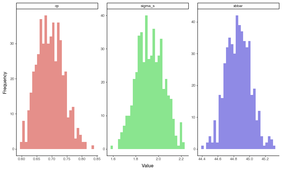
So cool! We've now generated the sampling distributions for our bootstrap statistics! Let's visualize the raw distributions to see those wicked cool bootstrapped sampling distributions:
# Create a more comprehensive bootstrap function that returns all statistics
def boot_comprehensive(seed=1):
    np.random.seed(seed)
    results = []
    for r in range(reps):
        sample = water.sample(n=len(water), replace=True)
        stat_s_b = (sample.groupby('time').apply(lambda d: pd.Series({
            'xbar': d['temp'].mean(),
            's': d['temp'].std(),
            'n_w': len(d)
        })).reset_index())

        xbbar_b = stat_s_b['xbar'].mean()
        sigma_s_b = (stat_s_b['s']**2).mean()**0.5
        cp_b = cp(sigma_s_b, upper=limit_upper, lower=limit_lower)

        results.append({
            'rep': r,
            'xbbar': xbbar_b,
            'sigma_s': sigma_s_b,
            'cp': cp_b
        })

    return pd.DataFrame(results)

# Generate bootstrap data
bootstrap_data = boot_comprehensive()

# Reshape for plotting
plot_data = []
for _, row in bootstrap_data.iterrows():
    plot_data.extend([
        {'type': 'xbbar', 'value': row['xbbar']},
        {'type': 'sigma_s', 'value': row['sigma_s']},
        {'type': 'cp', 'value': row['cp']}
    ])

plot_df = pd.DataFrame(plot_data)

# Create the plot
g = (ggplot(plot_df, aes(x='value', fill='type')) +
     geom_histogram(bins=30, alpha=0.7) +
     facet_wrap('~type', scales='free') +
     theme_classic(base_size=12) +
     labs(x='Value', y='Frequency') +
     theme(legend_position='none'))

# Save the plot
g.save('images/06_bootstrap_distributions.png', width=10, height=6, dpi=100)
Bootstrap Confidence Intervals
Now let's take our bootstrapped \( C_{p} \) statistics and estimate a confidence interval and standard error for this sampling distribution. Because we have the entire distribution, we can extract values at specific percentiles in the distribution using quantile(), rather than theoretical distributions.
print("Bootstrap Results for Cp:")
print(f"Original estimate: {bootstrap_results['cp'][0]:.3f}")
print(f"Bootstrap 95% CI: ({bootstrap_results['lower'][0]:.3f}, {bootstrap_results['upper'][0]:.3f})")
print(f"Bootstrap standard error: {bootstrap_results['se'][0]:.3f}")
This suggests a wider confidence interval than our normal distribution assumes by default - interesting!
Conclusion
You've successfully computed capability and performance indices (Cp, Cpk, Pp, Ppk) and their confidence intervals using both normal approximation and bootstrap methods in Python. These tools help us assess process capability and performance, providing insights into whether our processes meet specifications and how consistently they perform.