

p = 0.5049" on the F-test slide) is his own console read-out from the chapter's example and is kept for that reason. NO learning-check answer, quiz key or homework solution appears anywhere in this deck. No dates anywhere in this deck (ADR-029). -->
Rows of laboratory glassware on a bench, one flask in focus
Week: Design of Experiments

Workshop 12: ANOVA & Latin Squares

Applying T-tests and ANOVA
Tim Fraser
Tim Fraser, PhD
Research Associate, Systems Engineering
Cornell University
SYSEN 5300: Systems Engineering & Six Sigma
for Design and Operation of Reliable Systems
Learning Outcomes
Target with an arrow in the bullseye
  • Risk Analysis
    • Risk assessment and risk characterization
    • Failure Modes and Effects Analysis
    • Fault trees and event trees under uncertainty
  • Modeling Reliability
    • Component and system reliability
    • Physical acceleration models
    • Required function, stated conditions, specified time
Learning Outcomes
Target with an arrow in the bullseye
  • Quality Control
    • Six sigma and statistical process control
    • Detect when performance is deteriorating
    • Take corrective action in time
  • System Improvement
    • Optimize system design for reliability
    • Design of experiments
    • Response surfaces — innovation, problem solving, and discovery
Today's Class

  • Recap: Comparing 2 Groups
  • Comparing 3 Groups
  • Block Randomization with 3 Groups
  • Latin Squares
Rows of laboratory glassware on a bench, one flask in focus

Recap: Comparing 2 Groups


Workshop 12
Designing Experiments
Example 1
Comparing 2 Unpaired Samples with T-tests in R
  • An industrial process made varying yields from methods A and B.
  • Does B have a significantly better yield than A?
library(dplyr)
library(broom)

data = tibble(
  method = c("A","A","A","A","A","A","A","A","A","A",
             "B","B","B","B","B","B","B","B","B","B"),
  yield = c(89.7, 81.4, 84.5, 84.8, 87.3, 79.7, 85.1, 81.7, 83.7, 84.5,
            84.7, 86.1, 83.2, 91.9, 86.3, 79.3, 82.6, 89.1, 83.7, 88.5))
Example 1
Two flavors of unpaired t-test
# T-test assuming equal variance (unpaired)
t.test(formula = yield ~ method, data = data, var.equal = TRUE)

# T-test not assuming equal variance
t.test(formula = yield ~ method, data = data, var.equal = FALSE)
R console output of a two-sample t-test assuming equal variance
var.equal = TRUE
R console output of a Welch two-sample t-test
var.equal = FALSE
Example 2
Comparing Variance in 2 Groups with F-tests in R
  • An industrial process made varying yields from methods A and B.
  • Is the variance in yield for methods A vs. B significantly different?
library(dplyr)
library(broom)

data = tibble(
  method = c("A","A","A","A","A","A","A","A","A","A",
             "B","B","B","B","B","B","B","B","B","B"),
  yield = c(89.7, 81.4, 84.5, 84.8, 87.3, 79.7, 85.1, 81.7, 83.7, 84.5,
            84.7, 86.1, 83.2, 91.9, 86.3, 79.3, 82.6, 89.1, 83.7, 88.5))
Example 2
F test to compare two variances
# F test to compare two variances.
var.test(formula = yield ~ method, data = data)

# Are they significantly different? (No --> p = 0.5049)
R console output of var.test comparing the variance of yield between methods A and B
Example 3
Comparing 2 Paired Samples with T-tests in R
  • An industrial process made a series of paired products, each using method A and B.
  • Do the products made by B have a significantly better yield than A?
library(dplyr)
library(broom)

# When data comes in pairs, like this, we use paired t-tests.
data2 = tibble(
  yield_a = c(89.7, 81.4, 84.5, 84.8, 87.3, 79.7, 85.1, 81.7, 83.7, 84.5),
  yield_b = c(84.7, 86.1, 83.2, 91.9, 86.3, 79.3, 82.6, 89.1, 83.7, 88.5))
Example 3
Basic method for a paired t-test
t.test(data2$yield_a, data2$yield_b,
       paired = TRUE, var.equal = TRUE)
R console output of a paired t-test comparing yield_a and yield_b
Example 4
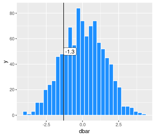
Permutation Test for Difference of Means
  • An industrial process made a series of paired products, each using method A and B.
  • Do the products made by B have a significantly better yield than A?
library(dplyr)
library(broom)

data = tibble(
  method = c("A","A","A","A","A","A","A","A","A","A",
             "B","B","B","B","B","B","B","B","B","B"),
  yield = c(89.7, 81.4, 84.5, 84.8, 87.3, 79.7, 85.1, 81.7, 83.7, 84.5,
            84.7, 86.1, 83.2, 91.9, 86.3, 79.3, 82.6, 89.1, 83.7, 88.5))
Example 4
Shuffle the labels 1000 times
perms = tibble(rep = 1:1000) %>%
  group_by(rep) %>%
  reframe(data) %>%
  group_by(rep) %>%
  mutate(yield = sample(yield, size = n(), replace = FALSE)) %>%
  group_by(rep) %>%
  summarize(dbar = mean(yield[method == "A"]) -
                   mean(yield[method == "B"]))
Example 4
Compare the observed difference to the null
# Get the observed difference of means
obs = data %>%
  summarize(dbar = mean(yield[method == "A"]) -
                   mean(yield[method == "B"]))

# 2-tailed percentage of random stats
# greater than the observed
mean( abs(perms$dbar) >= abs(obs$dbar) )
Histogram of 1000 permuted differences of means with the observed difference marked

Comparing 3 Groups


Workshop 12
Designing Experiments
Comparing 3 Groups
Case Study: Blood Coagulation Times
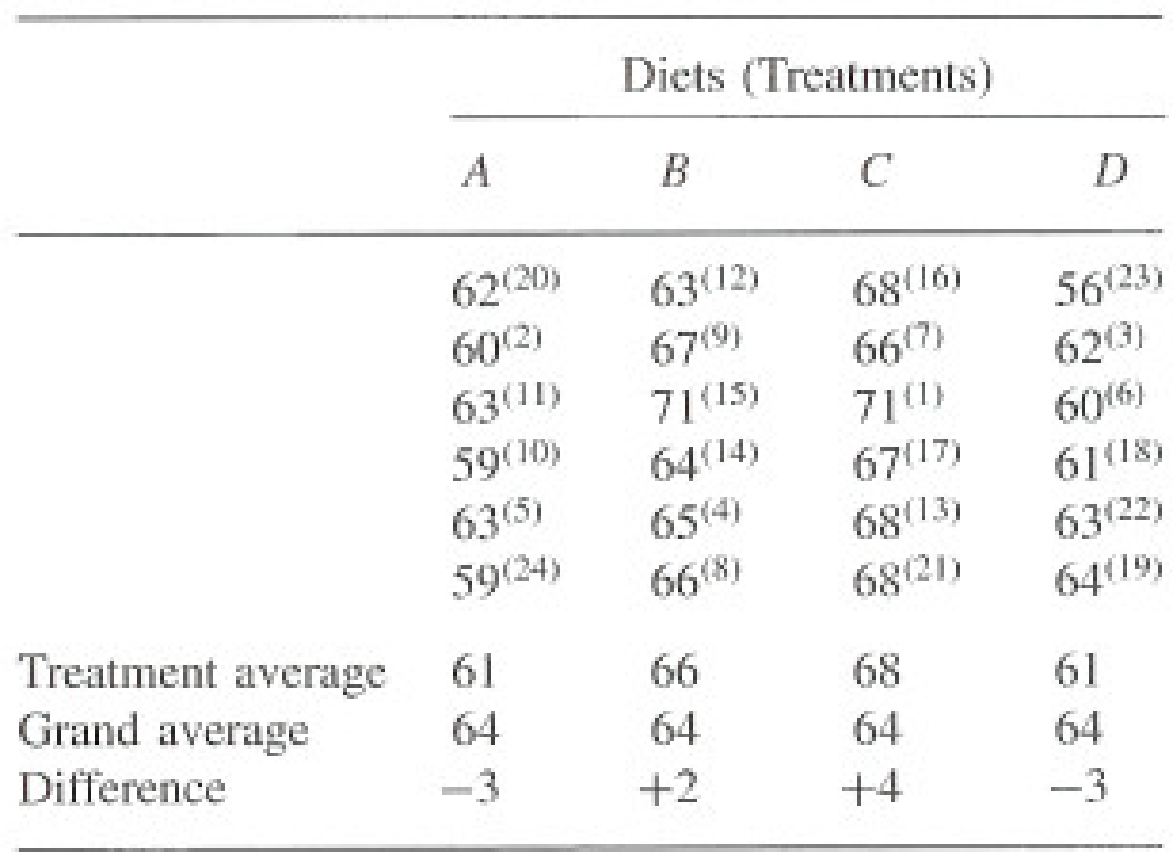
  • 24 animals receiving four different diets A, B, C, D.
  • Diets randomly assigned to animals.
  • Testing done in random order.
  • Is there real difference between the mean coagulation times for the 4 diets?
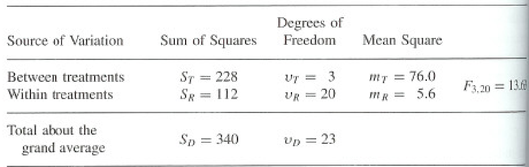
Analysis of Variance table for the coagulation experiment
Analysis of Variance (ANOVA) table
Table of coagulation times for 24 animals grouped by diet A, B, C and D
Comparing 3 Groups
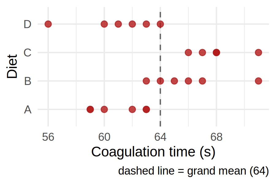
ANOVA: Analysis of Variance
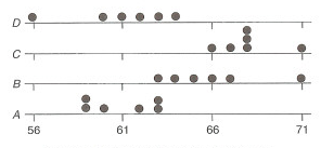
Scatter of coagulation times with the grand mean drawn against four group means
grand mean vs. four group means
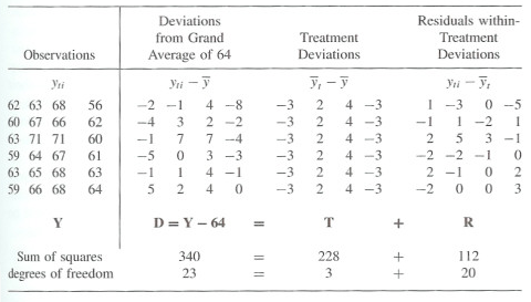
Decomposition of variation around the grand mean into group and within-group parts
  • Key Question: How much better are the groups at explaining variation than the grand mean?
Comparing 3 Groups
Calculating Deviations in ANOVA
Worked table of deviations of each observation from the grand mean and from its group mean
Diagram naming the total, explained and residual deviation for a single observation
Comparing 3 Groups
Three Sums of Squares
  • Total Sum of Squares measures the total variation in your data, using the grand mean as benchmark.
    • TSS = sum( (x - xbbar)^2 )
  • Residual Sum of Squares measures how much deviation remains within each treatment group. This is the unexplained error in your model.
    • RSS = sum( (x - xbar)^2 )
  • Explained Sum of Squares measures how much deviation was explained by your treatment group means.
    • ESS = TSS - RSS
Worked table of deviations of each observation from the grand mean and from its group mean
Comparing 3 Groups
Quantities of Interest in ANOVA
  • Mean Squares Explained: average variation explained, divided by k - 1 groups.
    • MSE = (TSS - RSS) / (k - 1)
  • Mean Squared Error: average variation unexplained, divided by n - k.
    • MSR = RSS / (n - k)
  • F-statistic: ratio of variation explained versus unexplained by your model.
    • F = MSE / MSR
n = sample size (24)     k = # of groups (4)
Comparing 3 Groups
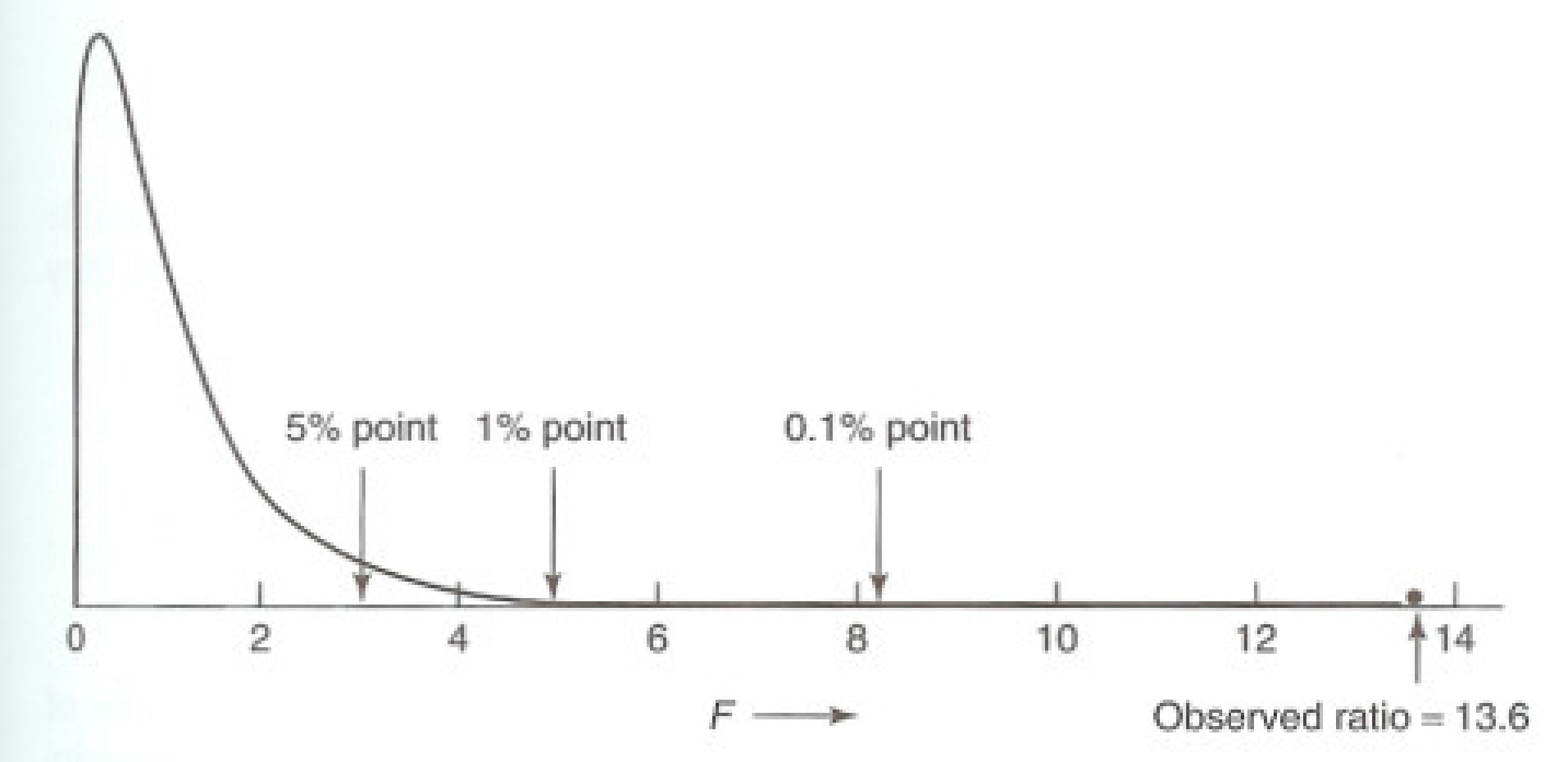
F-statistic in ANOVA
  • If the error is normally distributed (independence of observation assumption of regression)
  • Then MSE and MSR are independently distributed.
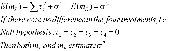
  • So, ratio F = MSE / MSR follows an F distribution.
  • F-statistic: How much better is your model than an intercept model alone? (grand mean)
Formula for the F ratio as mean squares explained over mean squared error
F distribution curve with the upper tail shaded
Example 5
Comparing 3+ group means with F-test in R
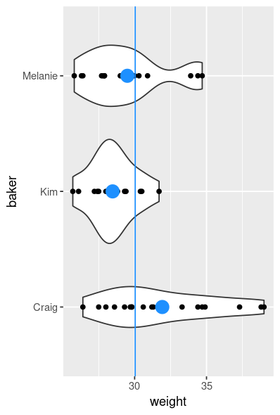
  • Craig, Kim, and Melanie work for a bakery, but Craig's donuts seem kinda weird.
  • Does the weight of these donuts vary significantly by the baker?
  • Calculate an F-statistic and evaluate its significance.
library(dplyr)
library(readr)
library(broom)

donuts = read_csv(
  "https://raw.githubusercontent.com/timothyfraser/sysen/main/workshops/donuts.csv")
Illustration of three bakers' donuts
Example 5
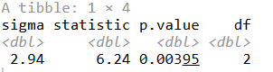
Route 1 — use lm()
donuts %>%
  summarize(lm(weight ~ baker) %>% glance()) %>%
  select(sigma, statistic, p.value, df)
R console output showing sigma, statistic, p.value and df from glance
Example 5
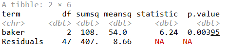
Route 2 — or use aov()
donuts %>%
  reframe(aov(weight ~ baker) %>% tidy())
R console output of a tidied analysis of variance table for weight by baker
Example 6
Comparing unequal group variances with K² test in R
  • Craig, Kim, and Melanie work for a bakery, but Craig's donuts seem kinda weird.
  • Does the variance in weight of these donuts vary significantly by baker? Calculate a K² statistic.
  • If so, we should NOT assume equal variance when doing ANOVA. Calculate your F statistic.
library(dplyr)
library(readr)
library(broom)

donuts = read_csv(
  "https://raw.githubusercontent.com/timothyfraser/sysen/main/workshops/donuts.csv")
Example 6
Homogeneity of Variance — Bartlett's test for K²
# Are the variances of my 3+ groups significantly different?
bartlett.test(weight ~ baker, data = donuts)

# If K-squared is significant,
# the differences in variance are significant.
R console output of Bartlett's test of homogeneity of variances
Example 6
ANOVA without the equal-variance assumption
donuts %>%
  summarize(
    oneway.test(weight ~ baker,
                data = donuts, var.equal = FALSE) %>% tidy())
R console output of a tidied one-way test that does not assume equal variance

Randomized Block Design with 3+ groups


Workshop 12
Designing Experiments
Comparing 3 Groups
Randomized Block Design
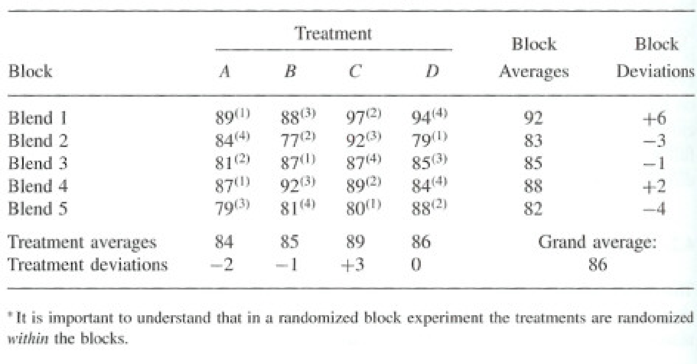
  • To thoroughly control for alternative explanations, we can randomly assign observations to treatments within blocks.
  • Example: Penicillin. Estimate effect of treatments accounting for blends.
  • N = 20 animals, five blends of 4.
Diagram of 20 animals split into five blends of four, each blend receiving treatments A, B, C and D
Comparing 3 Groups
Randomized Block Design (2)
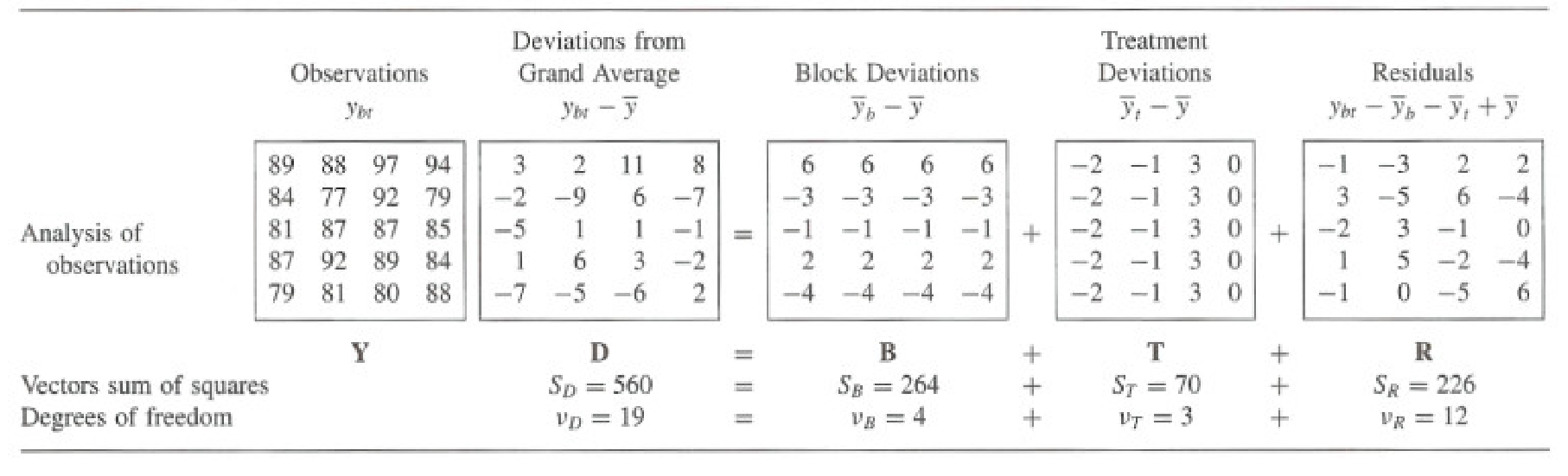
  • R = D - B - T; the vectors R, B, and T are mutually orthogonal.
Vector decomposition of the penicillin data into block, treatment and residual components
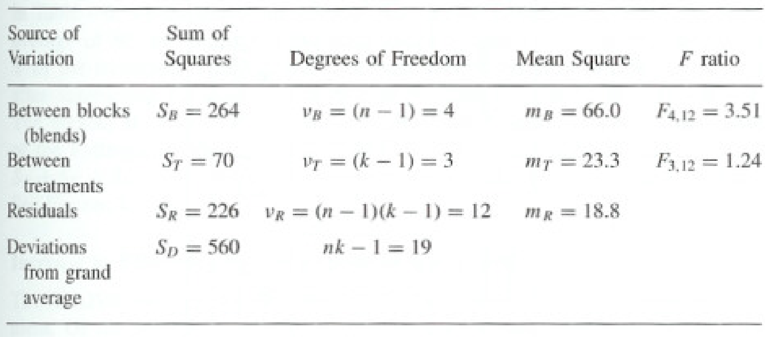
Analysis of variance table for the randomized block penicillin experiment
Comparing 3 Groups
Why Use Randomized Blocking?
  • Of the total sum of squares not associated with treatments or with the mean, almost 50% is just block-to-block variation.
  • If the experiment were arranged on a completely randomized basis with no blocks, the error variance would have been much larger.
  • With randomized blocks, error is much less: of the total of SD = 560, SB = 264 is removed by blocks.
  • Randomized block design greatly increased sensitivity of the experiment; now able to detect smaller treatment differences.
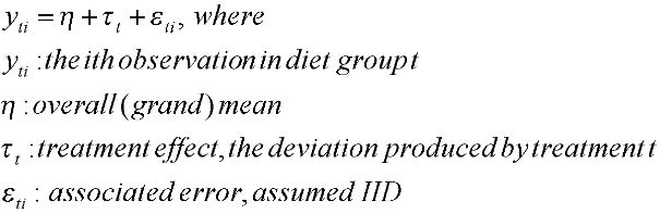
Algebraic formulation of the randomized block model
Formulation
Comparing 3 Groups
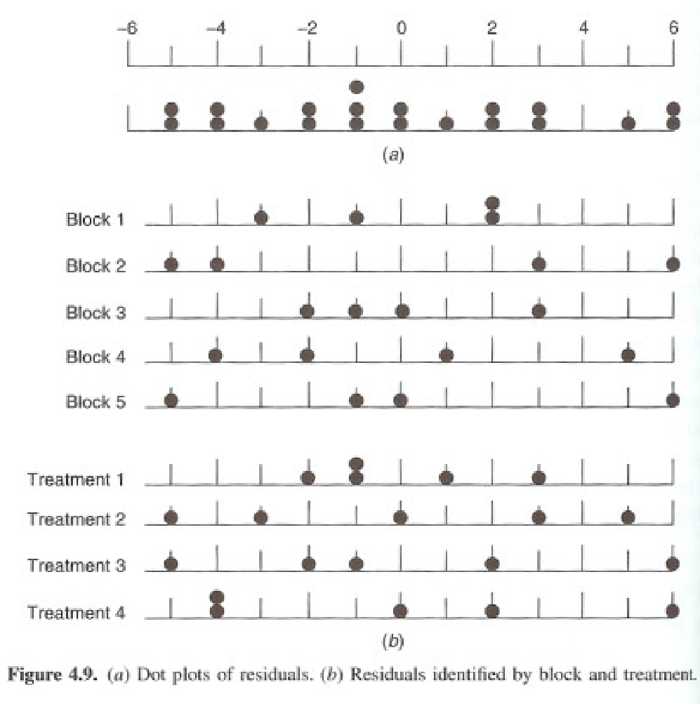
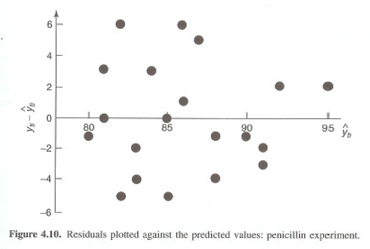
Randomized Block Design (4) — Diagnostic Tests
Diagnostic plots for the randomized block penicillin model
Residuals from the randomized block model plotted by blend and by treatment

Latin Squares


Workshop 12
Designing Experiments
Latin Squares
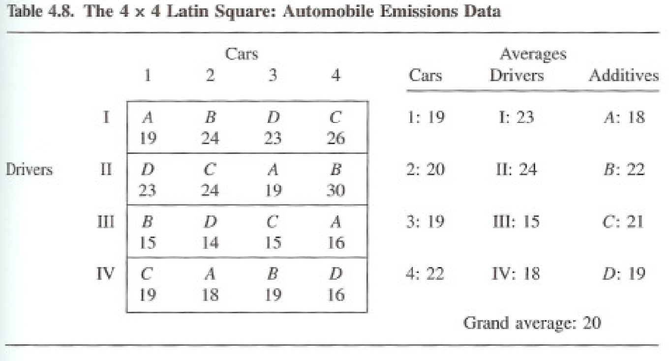
Using 2 Types of Blocks — Example: Air Pollution
  • How much does adding Chemical A, B, C, or D to gasoline reduce air pollution?
  • Hypothesized relationship: chemical type → air pollution.
  • Confounding variables: driver differences, car differences.
Latin square layout of four chemical treatments across four drivers and four cars
Latin Squares
The design rule
  • 4 treatments tested, 4 different drivers, 4 different cars.
  • 2 block factors: drivers & cars.
  • Latin Squares design helps eliminate differences in treatment comparisons that are just due to drivers or cars.
  • Each treatment (A, B, C, or D) randomly appears once per row (driver) and once per column (car).
Latin Squares
Using 2 Types of Blocks — Example: Air Pollution
Data table of emissions readings arranged as a Latin square of drivers by cars
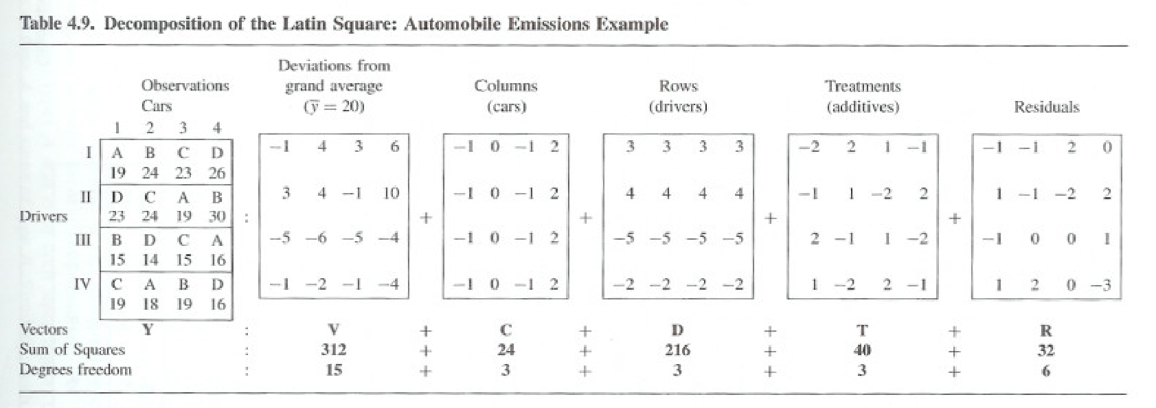
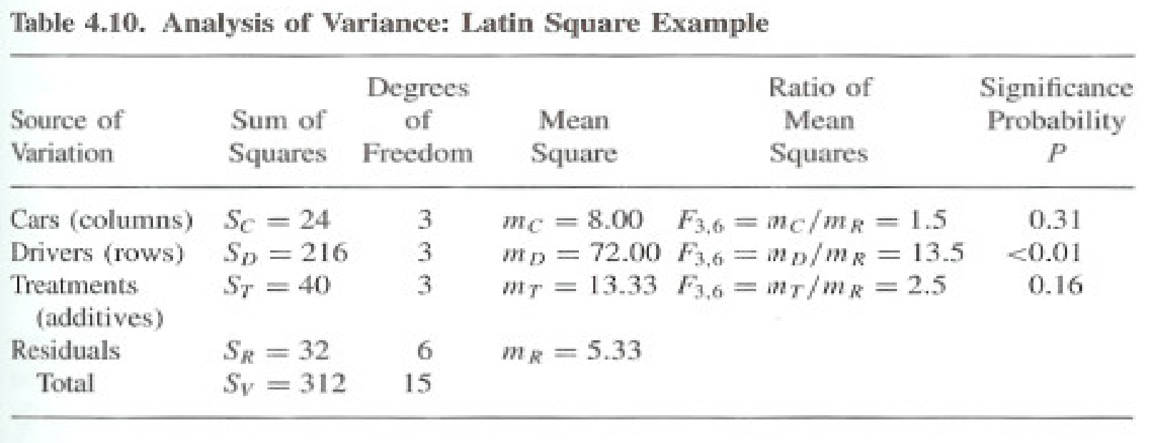
Analysis of variance table for the Latin square air pollution experiment
  • No convincing evidence for differences between the treatments.
  • Latin square design effective in eliminating variation due to drivers.
Latin Squares
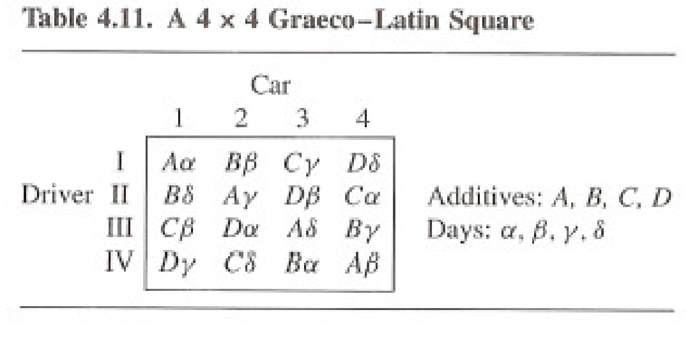
Using 3 Types of Blocks — Graeco-Latin Squares
  • A Graeco-Latin square is a k by k pattern.
  • Allows study of k treatments simultaneously, with 3 blocking variables, each at k levels.
  • Example: 1 extra blocking variable in car emissions — e.g. day of test.
Graeco-Latin square layout adding Greek-letter blocks to the Latin square of drivers and cars
Latin Squares
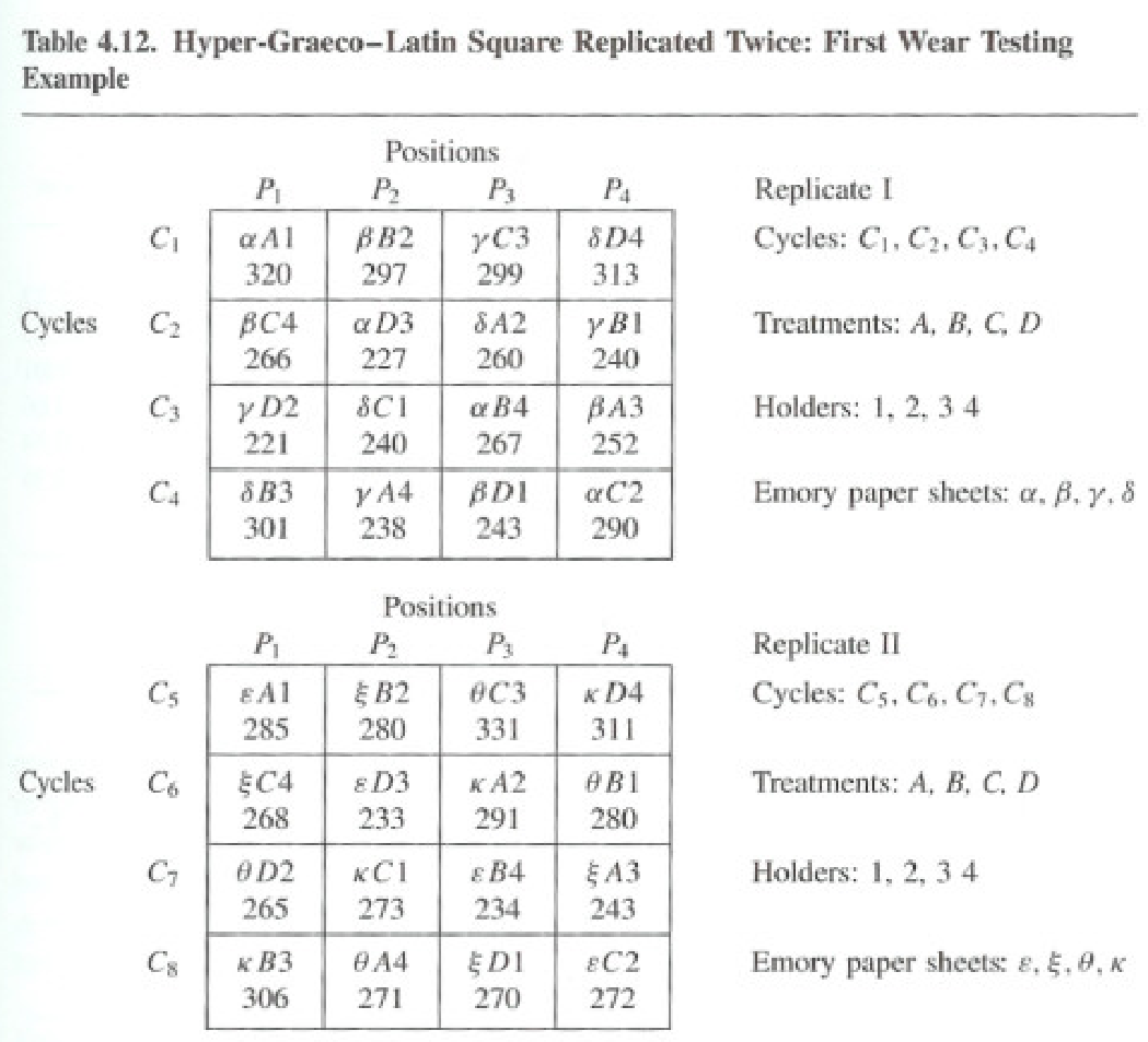
Using 3+ Types of Blocks — Example: Martindale Wear Tester
  • Machine used to test wearing quality of types of cloth.
  • Records weight loss from a test piece in 1 machine cycle (rubbed against a std. grade of emery paper).
  • Treatments: 4 types of cloth A, B, C, D.
  • Block Type 1: mounted in 4 specimen holders 1, 2, 3, 4.
  • Block Type 2: each holder can be in 1 of 4 positions P1, P2, P3, P4.
  • Block Type 3: each emery paper sheet (alpha, beta, gamma, delta) was cut into 4 quarters.
  • Objective: (1) make accurate comparison of the treatments; (2) understand variability caused by holders, positions, emery papers, and cycles.
Latin Squares
Hyper-Graeco Latin Squares — Example: Martindale Wear Tester
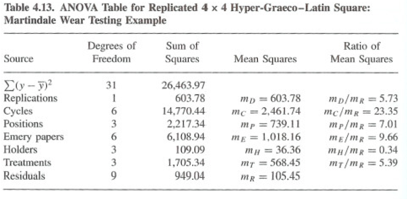
  • The design was effective both in removing sources of extraneous variation and in indicating their relative importance.
  • Because of the elimination of these disturbances, the residual variance was reduced by a factor of 8.
  • We could detect much smaller differences in treatment.
Hyper-Graeco-Latin square layout for the Martindale wear tester experiment
Latin Squares
Hyper-Graeco Latin Squares — what the analysis showed
  • The F-stat = 5.39 with 3, 9 DOF, significant at the 2% level.
  • By using a design which makes it possible to remove the effects of many larger disturbing factors, differences between treatments were made detectable.
  • The analysis identified the large contributions to the total variation due to cycles and to emery papers.
  • This suggested improvements, which later led to changes in the design of the machine.
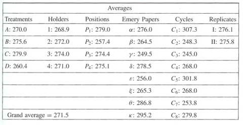
Analysis of variance table for the Martindale wear tester experiment Effect estimates for cloth, holder, position, emery paper and cycle
Latin Squares
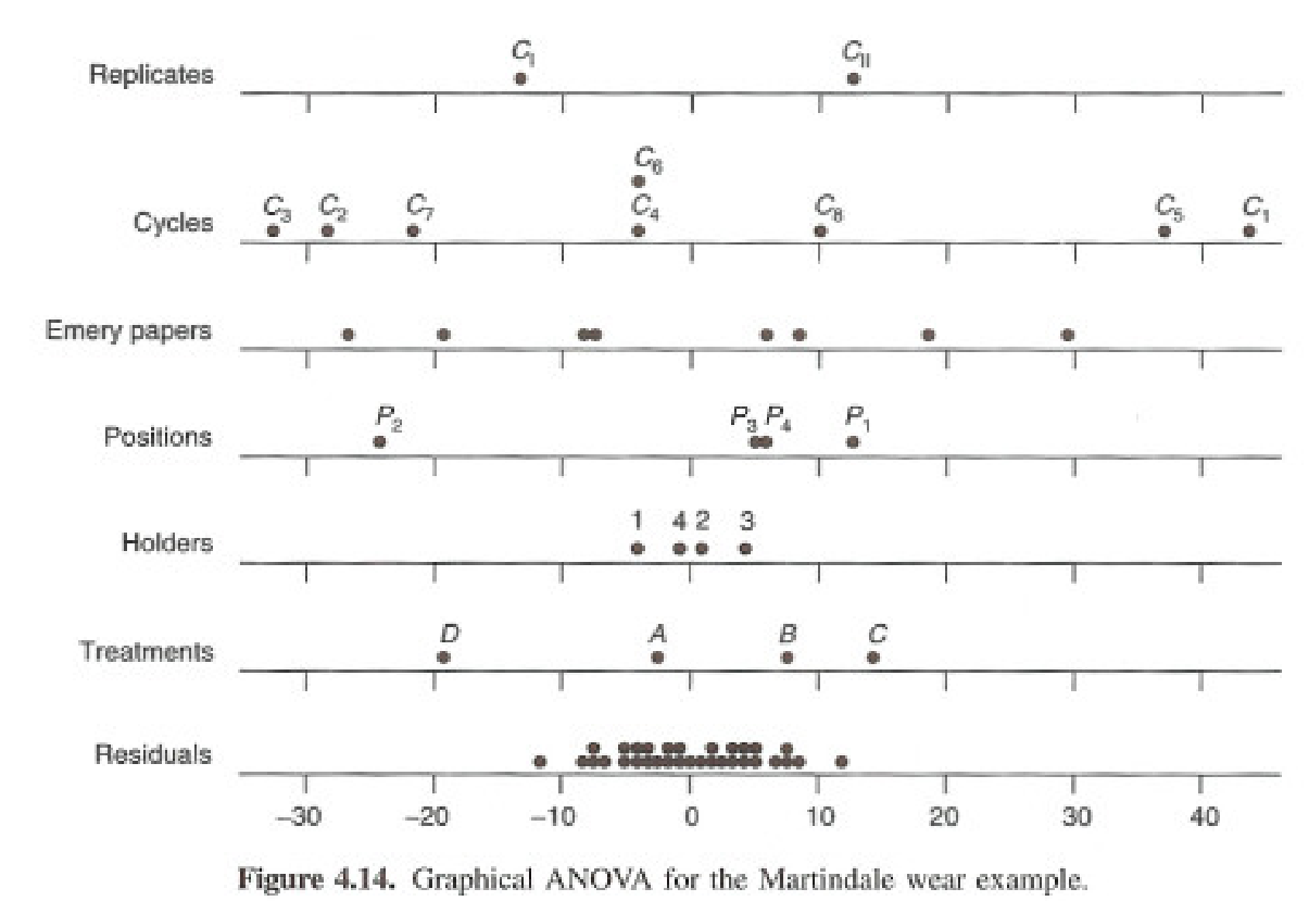
Hyper-Graeco Latin Squares — graphical analysis
  • In graphical analysis, position P2 gives much less wear than the others, indicating a need of improvement.
Dot plot of wear by holder position showing position P2 far below the others
Latin Squares
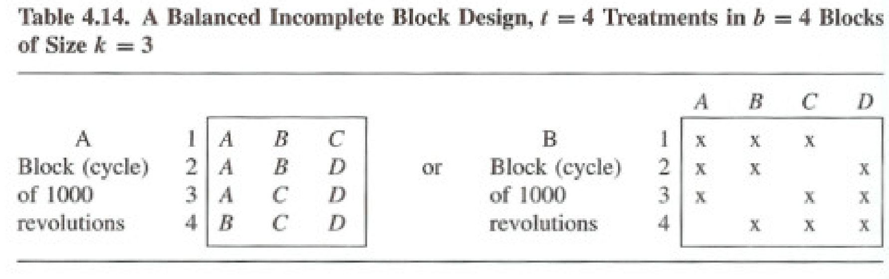
Balanced Incomplete Block Design
  • Suppose the Martindale wear tester allowed only three samples per cycle, but you had 4 treatments A, B, C, and D to compare.
  • 4 treatments but a block size of 3 — too small to accommodate all the treatments simultaneously → balanced incomplete block design.
  • Property: every pair of treatments occurs together in a block the same number of times.
Balanced incomplete block design layout of four treatments in blocks of three
Latin Squares
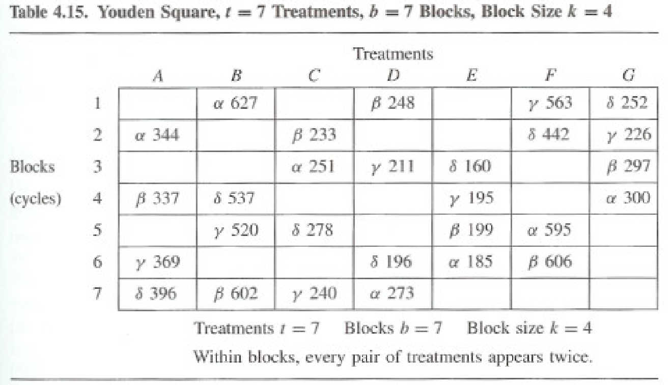
Doubly Balanced Incomplete Block Designs — Youden Squares
  • Compare 7 treatments in seven blocks of size 4 (e.g. test 7 types of cloth A–G).
  • But only 4 test pieces could be compared simultaneously in a single machine cycle.
  • Also had the opportunity to eliminate a second source of block variation: machine positions.
Youden square layout of seven treatments in seven blocks of four positions
Latin Squares
Factorial Design
  • How do we handle these wacky designs?
  • Learn more next week in Factorial Design!
Closing illustration pointing ahead to factorial design