Dense bundles of multicoloured fibres sweeping across a near-black ground
Week: Regression & Response Surfaces

Workshop 11: Regression in R

Modeling for System Improvement
Tim Fraser
Tim Fraser, PhD
Assistant Teaching Professor, Systems Engineering
Cornell University
SYSEN 5300: Systems Engineering & Six Sigma
for Design and Operation of Reliable Systems
Learning Outcomes
Target with an arrow in the bullseye
  • Risk Analysis
    • Risk assessment and risk characterization
    • Failure Modes and Effects Analysis
    • Fault trees and event trees under uncertainty
  • Modeling Reliability
    • Component and system reliability
    • Physical acceleration models
  • Quality Control
    • Six sigma and statistical process control
    • Catch performance slipping, in time to act
  • System Improvement
    • Design of experiments and response surfaces
    • Optimize system design for reliability

Today's Class

  • Reading Questions
  • Coding Demo
The big question:
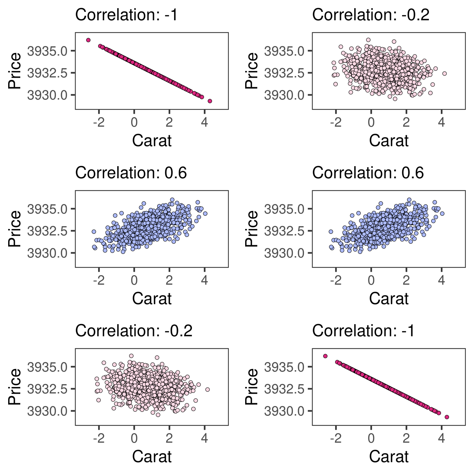
As X increases, what happens to Y?
Animated scatterplot: a cloud of points shifts from a negative to a positive relationship as the line of best fit swings with it

Reading Questions


Workshop 11
Activity: Explain It
Please complete the following steps
  1. Pick 2 reading questions from slides below.
  2. Copy the slide matching that function, and add it to our Slide Deck [Link]!
  3. Update it with your Group Number and your names.
  4. Fill in the slide with your answers to these questions.
  5. Take a screenshot of your slide and submit it in the CANVAS text submit box!

Two of the reading questions: 1. Reporting Effects, 10. Intercept with Categorical Variables.

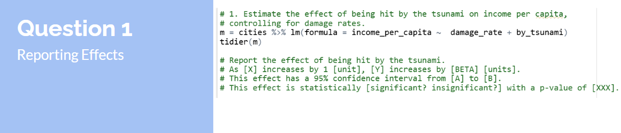
Explain It · Question 1
Question 1 card, Reporting Effects: estimate the effect of being hit by the tsunami on income per capita, controlling for damage rates, with m equals cities piped into lm of formula income per capita against damage rate plus by tsunami, then tidier of m; report the effect using the sentence frame as X increases by 1 unit, Y increases by BETA units, with a 95 percent confidence interval from A to B, statistically significant or insignificant with a p-value of XXX
Reading Question 1: Reporting Effects
Explain It · Question 10
Question 10 card, Intercept when using Categorical Variables: model the effect of each year on income; which year is not represented? The intercept represents that baseline category; cities dollar year piped into unique, then m equals cities piped into lm of formula income per capita against year; calculate the predicted income per capita from 2011 to 2017
Reading Question 10: Intercept with Categorical Variables
Activity: Explain It
Modeling Exercises
Load Data
library(dplyr)
library(readr)
library(broom)
library(texreg)
library(gtools)

cities = read_csv("workshops/jp_matching_experiment.csv") %>%
  # Tell R to treat year and pref as **ordered categories**
  mutate(year = factor(year),
         pref = factor(pref),
         by_tsunami = factor(by_tsunami, levels = c("Not Hit", "Hit")))

cities %>% glimpse()
import pandas as pd
import statsmodels.formula.api as smf
# lm() -> smf.ols(...).fit()

f = "workshops/jp_matching_experiment.csv"
cities = pd.read_csv(f)
# Treat year and pref as ordered categories
cities['year'] = cities['year'].astype('category')
cities['pref'] = cities['pref'].astype('category')
cities['by_tsunami'] = pd.Categorical(
  cities['by_tsunami'],
  categories=["Not Hit", "Hit"], ordered=True)

print(cities.info())
Modeling Exercises
Install Packages

You'll need these packages….

install.packages(c("dplyr", "readr", "broom", "texreg", "gtools"))
pip install pandas statsmodels plotnine
Modeling Exercises · Load Function
tidier = function(model, ci = 0.95, digits = 3){
  model %>%
    broom::tidy(conf.int = TRUE, conf.level = ci) %>%
    reframe(
      term = term,
      estimate = estimate %>% round(digits),
      se = statistic %>% round(digits),
      statistic = statistic %>% round(digits),
      p_value = p.value %>% round(digits),
      stars = p.value %>% gtools::stars.pval(),
      upper = conf.high %>% round(digits),
      lower = conf.low %>% round(digits))
}
def tidier(model, ci = 0.95, digits = 3):
    b = model.conf_int(alpha = 1 - ci)
    out = pd.DataFrame({
      'term': model.params.index,
      'estimate': model.params.round(digits),
      'se': model.bse.round(digits),
      'statistic': model.tvalues.round(digits),
      'p_value': model.pvalues.round(digits),
      'lower': b[0].round(digits),
      'upper': b[1].round(digits)})
    out['stars'] = pd.cut(out['p_value'],
      [0, .001, .01, .05, .1, 1],
      labels = ['***', '**', '*', '.', ''])
    return out.reset_index(drop = True)


Coding Demo


Workshop 11
Coding Demo
Your Turn: R playground

Fit a regression in R — price explained by carat — live, in the browser.

Your Turn: Python playground

The same fit in Python — smf.ols() instead of lm().