A dark painting crossed by pastel red, orange, blue and yellow curves rising and levelling off
Week:  Factorial Design

Lesson 13: Factorial Design

Testing Multiple Hypotheses in 1 Experiment
Tim Fraser
Tim Fraser, PhD
Assistant Teaching Professor, Systems Engineering
Cornell University
SYSEN 5300: Systems Engineering & Six Sigma
for Design and Operation of Reliable Systems
Learning Outcomes
Target with arrow in the bullseye
  • Risk Analysis
    • Risk assessment and risk characterization
    • Failure Modes and Effects Analysis
    • Fault trees and event trees under uncertainty
  • Modeling Reliability
    • Component and system reliability
    • Physical acceleration models
    • Required function, stated conditions, specified time
    • One element of the broader risk analysis
Learning Outcomes
Target with arrow in the bullseye
  • Quality Control
    • Six sigma and statistical process control
    • Detect when performance is deteriorating
    • Take corrective action in time
  • System Improvement
    • Optimize system design for reliability
    • Design of experiments
    • Response surfaces — innovation, problem solving, and discovery

Today's lesson

  • Housekeeping
  • Factorial Design & Enumeration
  • Main Effects
  • Two-Way Effects
  • Three-Way Effects
  • Design Decisions
A corgi in a red sweater teaching equations at a chalkboard to a classroom of corgis
Figured you wouldn't mind me reusing this image again.

Housekeeping (1)

Want to make your poster/report extra glitzy?

I can give out shared project space on my Overleaf account to teams who want to code up their project in Latex.

Optional - not necessary

Want in? Ask in class or on Ed Discussion and I will add your team to a shared Overleaf project.
LaTeX is optional. A clean Word or Google Doc poster scores exactly the same.

Housekeeping (2)

You Choose!

What should we cover in our last week of class?

We've been very efficient this term and have a couple of open days.

Please fill out the topic poll by the deadline on the Canvas item.

On the ballot: monitoring & control systems · scaling up your code · data communication · AI for Six Sigma

Factorial Design and Enumeration


Lesson 13
Factorial Design
Factorial Design
What is Factorial Design?
Factorial design:
  • select a fixed number of “levels” of each of a number of factors (variables)
  • run experiments for all possible combinations.
Factors:
  • quantitative: temperature, concentration
  • qualitative: +2 types of catalysts, or presence/absence of a trait
  · Unblocked Arrangement · Blocked Arrangement
Comparing 2 entities · T-test · Randomized blocking
Comparing k entities · ANOVA · Factorial Design
Factorial Design
What is Factorial Design?
Importance of 2-level factorial designs
  • few runs per factor;
  • easy interpretation;
  • direct further experimentation;
  • designs can be suitably augmented;
  · Unblocked Arrangement · Blocked Arrangement
Comparing 2 entities · T-test · Randomized blocking
Comparing k entities · ANOVA · Factorial Design
Factorial Design
Why? The Effects Table
Example A: All Effects with Pooled Standard Error
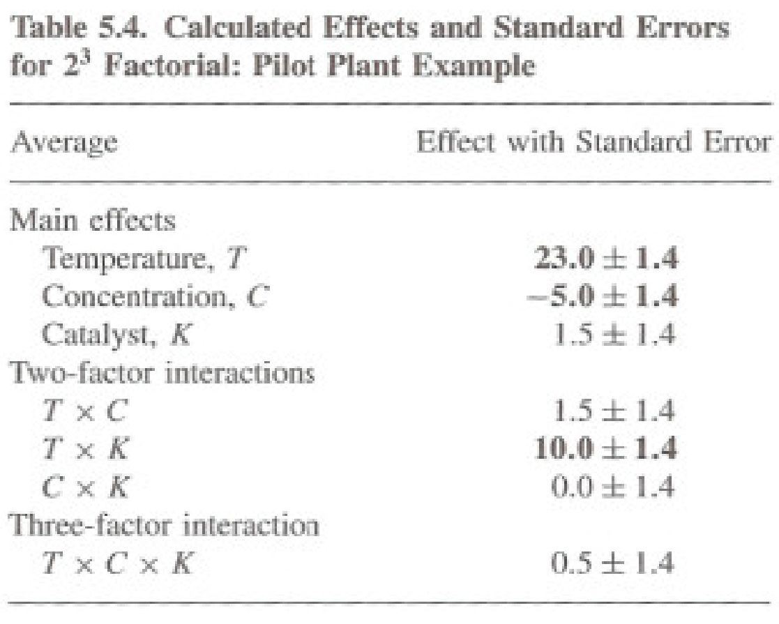
Table 5.4: calculated effects and standard errors for the 2 to the 3 factorial pilot plant example — main effects of temperature 23.0, concentration -5.0 and catalyst 1.5, two-factor interactions T by C 1.5, T by K 10.0, C by K 0.0, and three-factor interaction T by C by K 0.5, each plus or minus 1.4
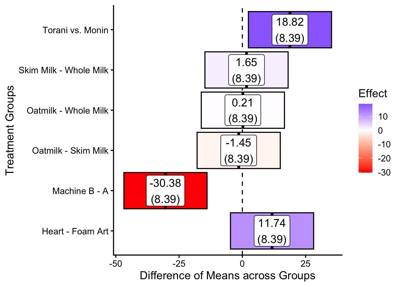
Example B: Direct Effects with Pooled Standard Error
Bar chart of differences of means across treatment groups: Torani vs Monin 18.82, skim minus whole milk 1.65, oatmilk minus whole milk 0.21, oatmilk minus skim milk -1.45, machine B minus A -30.38, heart minus foam art 11.74, each with a pooled standard error of 8.39
Factorial Design
Factorial Enumeration
Listing out all possible combinations of factor levels
  • ensures ~equal variance across treatment groups
  • view full range of variation
Use expand_grid() in tidyr package
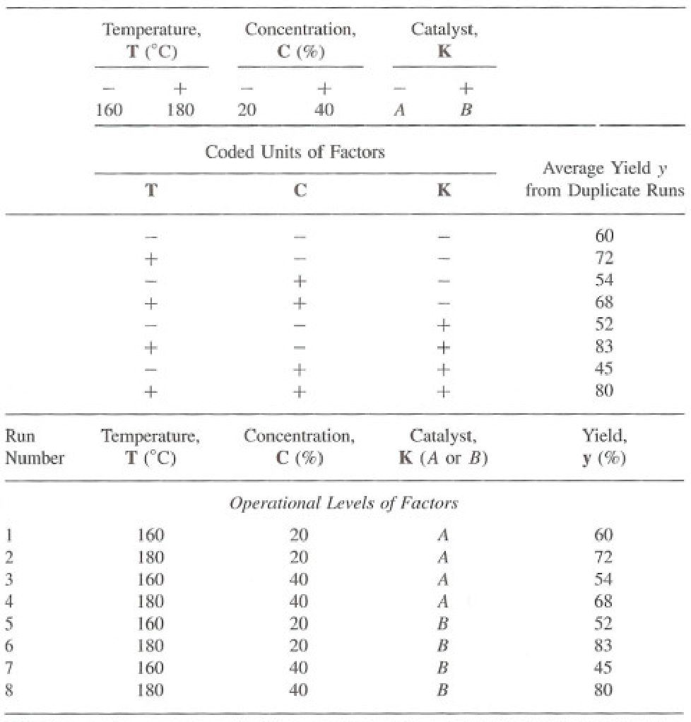
Pilot plant table: coded units of factors T, C and K with average yield y from duplicate runs, and the operational levels of factors for runs 1 to 8
Factorial Design
Factorial Enumeration
library(dplyr)
library(tidyr)

# Get full factorial grid of combinations
grid = expand_grid(
  # Catalyst K
  k = c("A", "B"),
  # Concentration C
  c = c(20, 40),
  # Temperature t
  t = c(160, 180),
) %>%
  # order columns as shown in the example...
  mutate(run = 1:n()) %>%
  select(run, t, c, k)
Pilot plant table: coded units of factors T, C and K with average yield y from duplicate runs, and the operational levels of factors for runs 1 to 8

Example 1

Factorial Enumeration in R

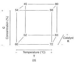
Encode this Factorial Design Cube as a dataframe!

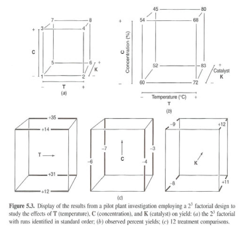
Factorial design cube of observed percent yields: 60, 72, 54 and 68 on the front face and 52, 83, 45 and 80 on the back, with axes for temperature T, concentration C and catalyst K
library(dplyr)
library(tidyr)

# Get full factorial grid of combinations
grid = expand_grid(
  # Catalyst K
  k = c("A", "B"),
  # Concentration C
  c = c(20, 40),
  # Temperature t
  t = c(160, 180),
) %>%
  # order columns as shown in the example...
  mutate(run = 1:n()) %>%
  select(run, t, c, k)

Example 1

Factorial Enumeration in R

Factorial design cube of observed percent yields: 60, 72, 54 and 68 on the front face and 52, 83, 45 and 80 on the back, with axes for temperature T, concentration C and catalyst K

Get every possible combination of Catalyst K, Concentration C, and Temperature T for your experiment.

Then, encode the outcomes as y!

# We run the experiment once and get these results
data = grid %>% mutate(y = c(60,72,54,68,52,83,45, 80))
  run       t     c k         y
<int> <dbl> <dbl> <chr> <dbl>
    1   160    20 A        60
    2   180    20 A        72
    3   160    40 A        54
    4   180    40 A        68
    5   160    20 B        52
    6   180    20 B        83
    7   160    40 B        45
    8   180    40 B        80

Main Effects


Lesson 13
Factorial Design
Factorial Design
23 Factorial Design
Pilot plant table: coded units of factors T, C and K with average yield y from duplicate runs, and the operational levels of factors for runs 1 to 8
Figure 5.3: display of the results from a pilot plant investigation employing a 2 to the 3 factorial design to study the effects of T, C and K on yield — panel a the factorial with runs in standard order, panel b observed percent yields, panel c the twelve treatment comparisons
Factorial Design
Estimating Main Effects
Steps: 1. Vary 1 variable, holding others constant  2. Get all within-group differences  3. Get average within-group difference
ID · T (C) · C (%) · K (A/B) · y (%)
1 · 160 · 20 · A · 60
2 · 180 · 20 · A · 72
3 · 160 · 40 · A · 54
4 · 180 · 40 · A · 68
ID · T (C) · C (%) · K (A/B) · y (%)
5 · 160 · 20 · B · 52
6 · 180 · 20 · B · 83
7 · 160 · 40 · B · 45
8 · 180 · 40 · B · 80
Factorial Design
Comparison of Concentrations, across all T & K groups (n = 4)  |  Effect of Concentration Change from 20 to 40%
Group · Concen. C · Temp T · Catalyst K · Effect (Cells) · Effect (Math) · d
a · 40/20 · 160 · A · y3 - y1 · 54 - 60 · -6
b · 40/20 · 180 · A · y4 - y2 · 68 - 72 · -4
c · 40/20 · 160 · B · y7 - y5 · 45 - 52 · -7
d · 40/20 · 180 · B · y8 - y6 · 80 - 83 · -3
Main (average) effect (d̄) of change in Concentration ΔC · (ya+ yb+ yc+yd) / n · (-6 + -4 + -7 + -3) / 4 · -5
Factorial Design
Estimating Main Effects Visually
Steps:
  1. Vary 1 variable, holding others constant
  2. Get all within-group differences
  3. Get average within-group difference
Factorial design cube of observed percent yields: 45, 80, 54, 68 on the top face and 52, 83, 60, 72 on the bottom, with axes for temperature T, concentration C and catalyst K
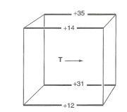
Cube of the four temperature comparisons: +35, +14, +31 and +12 along the T direction
Factorial Design
Comparison of Temperatures, across all C & K groups (n = 4)  |  Effect of Temperature Change from 160 to 180
Group · Concen. C · Temp T · Catalyst K · Effect (Cells) · Effect (Math) · d
a · 20 · 180/160 · A · y2 - y1 · 72 - 60 · +12
b · 20 · 180/160 · A · y6 - y5 · 83 - 52 · +31
c · 40 · 180/160 · B · y4 - y3 · 68 - 54 · +14
d · 40 · 180/160 · B · y8 - y7 · 80 - 45 · +35
Main (average) effect (d̄) of change in Temperature ΔT · (ya+ yb+ yc+yd) / n · (12 + 31 + 14 + 35) / 4 · +23

Example 2

Coding Main / Direct Effects

Estimate the direct effects of Concentration, Temperature, and the Catalyst from this experiment, coding in R.

Factorial design cube of observed percent yields with axes for temperature T, concentration C and catalyst K
Starting with our 'data' data.frame from Example 1…
  run       t     c k         y
<int> <dbl> <dbl> <chr> <dbl>
    1   160    20 A        60
    2   180    20 A        72
    3   160    40 A        54
    4   180    40 A        68
    5   160    20 B        52
    6   180    20 B        83
    7   160    40 B        45
    8   180    40 B        80
Example 2
Coding Main / Direct Effects
# Calculate the direct (one-way) treatment effects
data %>%
  summarize(
    dbar_c = mean( y[c==40] - y[c==20] ),
    dbar_t = mean( y[t== 180] - y[t==160] ),
    dbar_k = mean( y[k== "B"] - y[k=="A"] )
  )
dbar_c dbar_t dbar_k
 <dbl>  <dbl>  <dbl>
    -5     23    1.5

Two-Way Interaction Effects


Lesson 13
Factorial Design
Factorial Design
Two-Way Interactions
  • When two factors have a coupled influence on y beyond their main effects
  • e.g., temperature and catalyst
  • measured by difference between the temperature effects at the plus and minus levels of the catalyst factor.
Factorial design cube of observed percent yields: 45, 80, 54, 68 on the top face and 52, 83, 60, 72 on the bottom, with axes for temperature T, concentration C and catalyst K
Factorial Design
Two-Way Interactions

ŷ1 = (Y180,B + Y160,A) / 2

80, 83   60, 54

ŷ0 = (Y160,B + Y180,A) / 2

52, 45   72, 68

d̄ = ŷ1 - ŷ0

Temp T · Catalyst A · Catalyst B
180  72, 68  80, 83
160  60, 54  52, 45

Example 3

Coding Two-Way Interaction Effects

Estimate the two-way interaction effects of Temperature T and Catalyst K together on the outcome, coding in R.

Factorial design cube of observed percent yields with axes for temperature T, concentration C and catalyst K
Starting with our 'data' data.frame from Example 1…
  run       t     c k         y
<int> <dbl> <dbl> <chr> <dbl>
    1   160    20 A        60
    2   180    20 A        72
    3   160    40 A        54
    4   180    40 A        68
    5   160    20 B        52
    6   180    20 B        83
    7   160    40 B        45
    8   180    40 B        80
Example 3
Coding Two-Way Interaction Effects
# Calculate the two-way treatment effects
data %>%
  reframe(
    xbar1 = y[ (t==180 & k=="B") | (t==160& k=="A") ] %>% mean(),
    xbar0 = y[ (t==160 & k=="B") | (t==180& k=="A")] %>% mean(),
    dbar = xbar1 - xbar0
  )
A tibble: 1 × 3
xbar1 xbar0  dbar
<dbl> <dbl> <dbl>
 69.2  59.2    10

Three-Way Interaction Effects


Lesson 13
Factorial Design
Factorial Design
Three-Way Interactions
  • When 3 factors have a coupled influence
  • e.g., temperature, catalyst, AND concentration
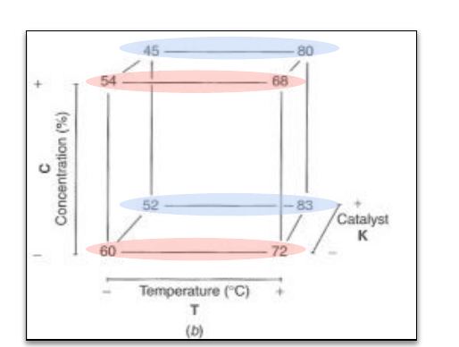
  • measured by average difference between the temperature*concentration effects at the plus and minus levels of the catalyst factor.
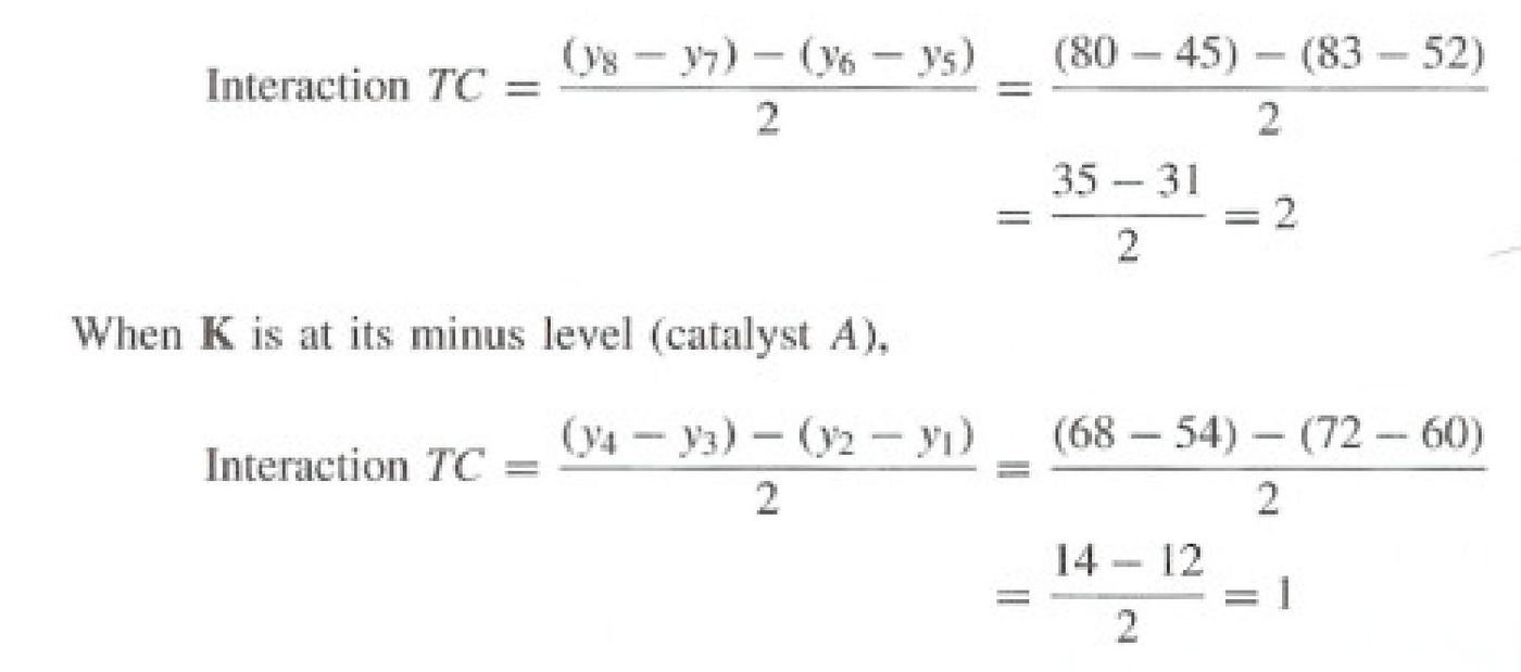
Interaction TC equals the quantity y8 minus y7 minus the quantity y6 minus y5, all over 2, equals 80 minus 45 minus 83 minus 52, over 2, equals 35 minus 31 over 2 equals 2; when K is at its minus level, catalyst A, interaction TC equals y4 minus y3 minus y2 minus y1 over 2 equals 68 minus 54 minus 72 minus 60 over 2 equals 14 minus 12 over 2 equals 1
  • Three-factor interaction of T, C, and K. TCK=(2-1)/2=0.5
Factorial design cube with the 45-80 and 52-83 edges circled in blue and the 54-68 and 60-72 edges circled in pink, marking the temperature by concentration comparisons at each level of catalyst K

Example 4

Coding Three-Way Interaction Effects

Estimate the three-way interaction effects of Temperature T, Catalyst K, and Concentration C together on the outcome, coding in R.

Factorial design cube of observed percent yields with axes for temperature T, concentration C and catalyst K
Starting with our 'data' data.frame from Example 1…
  run       t     c k         y
<int> <dbl> <dbl> <chr> <dbl>
    1   160    20 A        60
    2   180    20 A        72
    3   160    40 A        54
    4   180    40 A        68
    5   160    20 B        52
    6   180    20 B        83
    7   160    40 B        45
    8   180    40 B        80
Example 4
# Now get the average difference between these interactions
data %>%
  reframe(
    # Get the TC interaction when K is A
    d1a = y[t==180&k=="A"&c==40] - y[t==160&k=="A"&c==40],
    d0a = y[t==180&k=="A"&c==20] - y[t==160&k=="A"&c==20],
    dbar_a = (d1a - d0a)/2,

    # Get the TC interaction when K is B
    d1b = y[t==180&k=="B"&c==40] - y[t==160&k=="B"&c==40],
    d0b = y[t==180&k=="B"&c==20] - y[t==160&k=="B"&c==20],
    dbar_b = (d1b - d0b)/2,

    # Get three way interaction effect
    dbar = (dbar_b - dbar_a) / 2
  )
  d1a   d0a dbar_a   d1b   d0b dbar_b  dbar
<dbl> <dbl>  <dbl> <dbl> <dbl>  <dbl> <dbl>
   14    12      1    35    31      2   0.5

Factorial Design
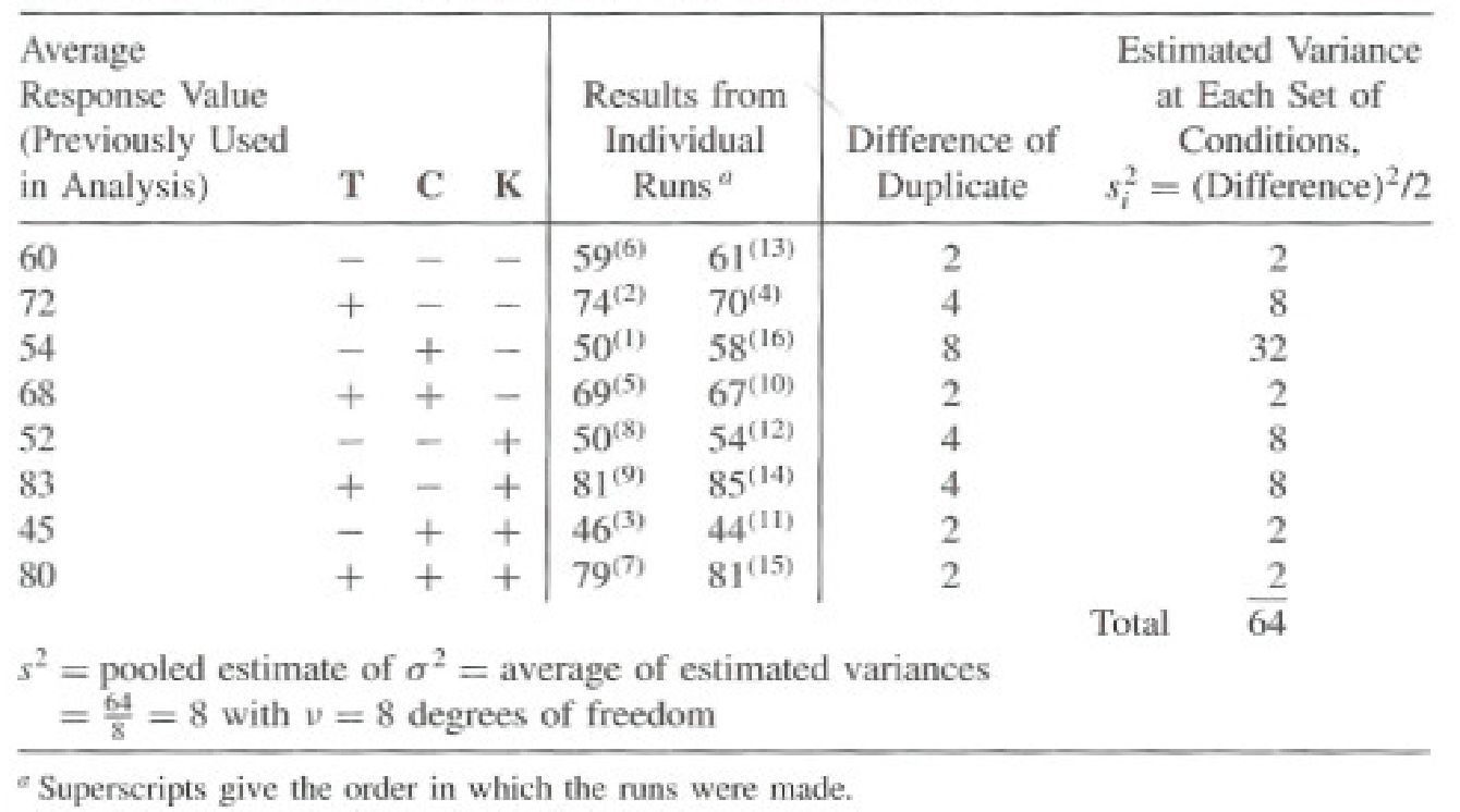
Genuine Replicate Runs
  • Good experiments rely on not just 1 replicates, but many replicates
  • Allows us to estimate standard errors
Table of average response values with the results from individual duplicate runs, the difference of duplicates, and the estimated variance at each set of conditions, totalling 64 with a pooled estimate s squared of 8 on 8 degrees of freedom

Each estimated effect T, C, K, TC, … is a difference between two averages of 8 obs., the variance of effect

v = 8 degrees of freedom  (2 - 1)*8

ndifferences = 8, groups = 2

Var(Effect)=(⅛ + ⅛) s2 = 2

SE(Effect)=1.4

Factorial Design
Genuine Replicate Runs
  • Randomization of run order ensures replication is genuine
  • i.e., variation between runs with same experimental conditions reflects total run-to-run variability
  • requires all the steps all over again.
Table of average response values with the results from individual duplicate runs, the difference of duplicates, and the estimated variance at each set of conditions, totalling 64 with a pooled estimate s squared of 8 on 8 degrees of freedom
Factorial Design
Standard Errors of Effects
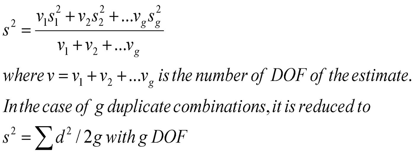
  • In general, if each factor combination was replicated, a pooled estimate of the experimental run variance from g factor combinations:
s squared equals v1 s1 squared plus v2 s2 squared plus dot dot dot vg sg squared, all over v1 plus v2 plus dot dot dot vg, where v equals v1 plus v2 plus dot dot dot vg is the number of DOF of the estimate; in the case of g duplicate combinations it is reduced to s squared equals the sum of d squared over 2g with g DOF
  • What is s2 in pilot plant example? What is variance (effect) and SE (effect)?
Factorial Design
Effects Tables
  • It is important to determine which effects are almost certainly real and which might readily be explained by chance.
  • A rough rule is that effects greater than 2-3 times their standard error are not easily explained by chance alone.
Table 5.4: calculated effects and standard errors for the 2 to the 3 factorial pilot plant example — main effects of temperature 23.0, concentration -5.0 and catalyst 1.5, two-factor interactions T by C 1.5, T by K 10.0, C by K 0.0, and three-factor interaction T by C by K 0.5, each plus or minus 1.4

Coding Demo


Lesson 13
Factorial Design
A stack of cartoon corgis piled into a pyramid