4 Workshop: System Reliability

In this tutorial, we’re going to learn how to conduct Reliability Analysis (also known as Survival Analysis) in R.

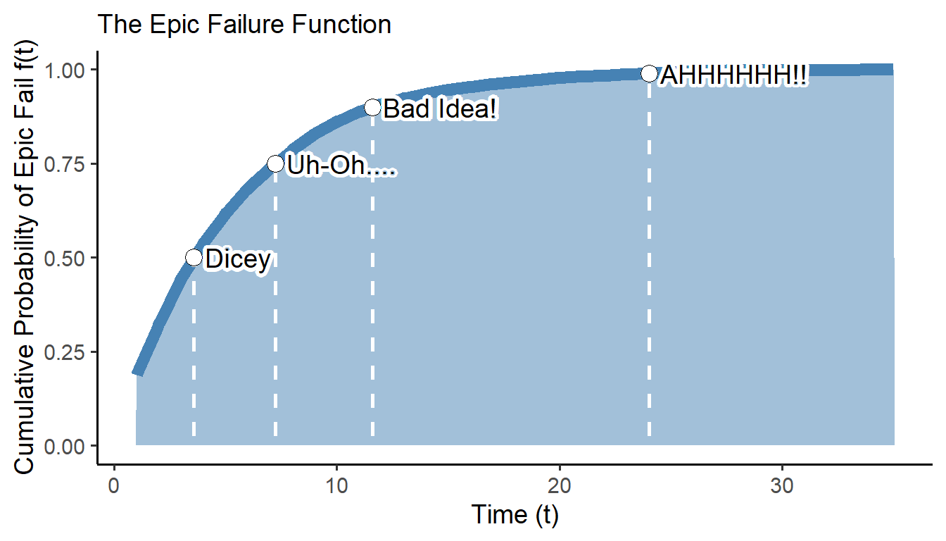
(#fig:img_epic_fail)Figure 1. Why We Do Reliability Analysis

Getting Started

Packages

library(tidyverse)
library(broom)
library(DiagrammeR)

4.1 Concepts

In Reliability/Survival Analysis, our quantity of interest is the amount of time it takes to reach a particular outcome (eg. time to failure, time to death, time to market saturation, etc.) Let’s learn how to approximate them in R!

4.1.1 Life Distributions

All technologies, operations, etc. have a ‘lifetime distribution’. If you took a sample of, say, cars in New York, you could measure how long each car functioned properly (its life-span), and build a Lifetime Distribution from that vector.

# Let's imagine a normally distributed lifespan for these cars...
lifespan <- rnorm(100, mean = 5, sd = 1)

The lifetime distribution is the probability density function telling us how frequently each potential lifespan is expected to occur.

# We can build ourself the PDF of our lifetime distribution here
dlife <- lifespan %>% density() %>% tidy() %>% approxfun()

In contrast, the Cumulative Distribution Function (CDF) for a lifetime distribution tells us, for any time $t$, the probability that a car will fail by time $t$.

# And we can build the CDF here
plife <- lifespan %>% density() %>% tidy() %>% 
  mutate(y = cumsum(y) / sum(y)) %>% approxfun()

Having built these functions for our cars, we can generate the probability (PDF) and cumulative probability (CDF) of failure across our observed vector of car lifespans, from ~3.11 to ~7.74.

Reliability or Survival Analysis is concerned with the probability that a unit (our car) will still be operating by a specific time $t$, representing the percentage of all cars that will survive to that point in time. So let’s also calculate 1 - cumulative probability of failure.

mycars <- tibble(
  time = seq(min(lifespan), max(lifespan), by = 0.1),
  # Get probability of failing at time time
  prob = time %>% dlife(),
  # Get probability of failing at or before time t
  prob_cumulative = time %>% plife(),
  # Get probability of surving past time t 
  # (NOT failing at or before time t) 
  prob_survival = 1 - time %>% plife())

Let’s plot our three curves!

ggplot() +
  # Make one area plot for Cumulative Probability (CDF)
  geom_area(data = mycars, 
            mapping = aes(x = time, y = prob_cumulative, 
                          fill = "Cumulative Probability"), alpha = 0.5) +
  # Make one area plot for Relibability
  geom_area(data = mycars, 
            mapping = aes(x = time, y = prob_survival, 
                          fill = "Reliability (Survival)"), alpha = 0.5) +
  # Make one area plot for Probability (PDF)
  geom_area(data = mycars,
            mapping = aes(x = time, y = prob, 
                          fill = "Probability"), alpha = 0.5) +
  theme_classic() +
  theme(legend.position = "bottom") +
  labs(x = "Lifespan of Car", y = "Probability",
       subtitle = "Example Life Distributions")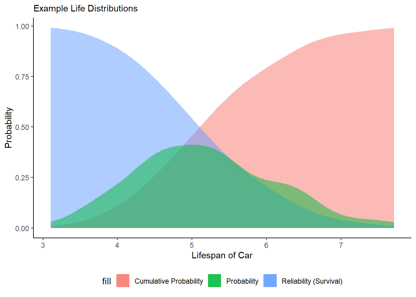

Figure 4.1: Figure 2. Life Distributions of a Fleet of Cars

This new reliability function allows us to calculate 2 quantities of interest:

expected (average) number of cars that fail up to time $t$.
total cars expected to still operate after time $t$.

4.1.2 Example: Airplane Propeller Failure!

Suppose Lockheed Martin purchases 800 new airplane propellers. When asked about the failure rate, the seller reports that every 1500 days, 2 of these propellers are expected to break. Using this, we can calculate $m$, the mean time to fail!

\[ \lambda \ t = t_{days} \times \frac{2 \ units}{1500 \ days} \ \ \ and \ \ \ m = \frac{1500}{2} = 750 \ days \] This lets us generate the failure rate $F(t)$, also known as the Cumulative Distribution Function, and we can write it up like this.

\[ CDF(t) = F(t) = 1 - e^{-(2t/1500)} = 1 - e^{-t/750} \] What’s pretty cool is, we can tell R to make a matching function fplane(), using the function() command.

# For any value `t` we supply, do the following to that `t` value.
fplane = function(t){ 1 - exp( -1*(t / 750)) }

Let’s use our function fplane() to answer our Lockheed engineers’ questions.

What’s the probability a propeller will fail by t = 600 days? By t = 5000 days?

fplane(t = c(600, 5000))

## [1] 0.5506710 0.9987274

Looks like 55% will fail by 600 days, and 99% fail by 5000 days.

What’s the probability a propeller will fail between 600 and 5000 days?

fplane(t = 5000) - fplane(t = 600)

## [1] 0.4480563

~45% more will fail between this period.

What percentage of new propellers will work more than 6000 days?

1 - fplane(t = 6000)

## [1] 0.0003354626

0.03% will survive past 6000 days.

If Lockheed uses 300 propellers, how many will fail in 1 year? In 3 years?

# Given a sample of 300 propellers,
n <- 300
# We project n * fplane(t = 362.25) will fail in 1 year (365.25 days)
# that's ~115 propellers.
n*fplane(t = 365.25)

## [1] 115.6599

# We also prject that n * fplane(t = 3 * 362.25) will fail in 3 years
# that's ~230 propellers!
n*fplane(t = 3*365.25)

## [1] 230.3988

Pretty powerful!

Learning Check 1

Question

(#fig:img_phone)Figure 3. Exploding Phones! (True Story)

Hypothetical: Samsung is releasing a new Galaxy phone. But after the 2016 debacle of exploding phones, they want to estimate how likely it is a phone will explode (versus stay intact). Their pre-sale trials suggest that every 500 days, 5 phones are expected to explode. What percentage of phones are expected to work after more than 6 months? 1 year?

[View Answer!]

Using the information above, we can calculate the mean time to fail m, the rate of how many days it takes for an average unit to fail.

days <- 500
units <- 5
m <- days / units
# Check it!
m

## [1] 100

We can use m to make our explosion function fexplode(), which in this case, is our (catastrophic) failure function $f(t)$!

\[ CDF(days) = Explode(days) = 1 - e^{-(days \times \frac{1 \ unit}{100 \ days})} = 1 - e^{-0.01 \times days} \]

fexplode = function(days){ 1 - exp(-1*days*0.01) }

Then, we can calculate $r(t)$, the cumulative probability that a phone will not explode after $t$ days.

Let’s answer our questions!

What percentage of phone are expected to survive 6 months?

# What percent
1 - fexplode(365.25 / 2)

## [1] 0.1610162

What percentage of phone are expected to survive 1 year?

1 - fexplode(365.25)

## [1] 0.02592623

4.2 Joint Probabilities

Two extra rules of probability can help us understand system reliability.

4.2.1 Multiplication Rule

probability that $n$ units with a reliability function $R(t)$ survive past time $t$ is multiplied, because of conditional probability, to equal $R(t)^{n}$..

Figure 4.2: Figure 4. Oops.

For example, there’s a 50% chance that 1 coffee cup breaks at local coffeeshop Coffee Please! every 6 months (180 days). Thus, the mean number of days to cup failure is $m = \frac{180 \ days}{ 1 \ cup \times 0.50 \ chance} = 360 \ days$, while the relative frequency (probability) that a cup will break is $ = $.

fcup = function(days){ 1 - exp( -1*(days/360))}
# So the probability that 1 breaks within 100 days is XX percent
fcup(100)

## [1] 0.2425349

And let’s write out a reliability function too, based on our function for the failure function.

# Notice how we can reference an earlier function fcup in our later function? Always have to define functions in order.
rcup = function(days){ 1 - fcup(days) }
# So the probability that 1 *doesn't* break within 100 days is XX perecent
rcup(100)

## [1] 0.7574651

But the probability that two break within 100 days is…

fcup(100) * fcup(100)

## [1] 0.05882316

And the probability that 5 break within 100 days is… very small!

fcup(100)^5

## [1] 0.0008392106

4.2.2 Compliment Rule

The probability that at least 1 of $n$ units fails by time $t$ is $1 - R(t)^{n}$.

So, if Coffee Please! buys 2 new cups for their store, the probability that at least 1 unit breaks within a year is…

1 - rcup(days = 365.25)^2

## [1] 0.868555

While if they buy 5 new cups for their store, the chance at least 1 cup breaks within a year is…

1 - rcup(days = 365.25)^5

## [1] 0.9937359

4.3 Types of Failure Rates

4.3.1 Hazard Rate Function

But if a unit has survived up until now, shouldn’t its odds of failing change? We can express this as:

\[ P(Fail \ Tomorrow | Survive \ until \ Today) = \frac{ F(days + \Delta days) - F(days) }{ \Delta days \times R(days)} = \frac{ F(days + 1 ) - F(days) }{ 1 \times R(days)} \] Local coffeeshop Coffee Please! also has a lucky mug, which has stayed intact for 5 years, despite being dropped numerous times by patrons. Coffee Please!’s failure rate suggests they had a 99.3% chance of it breaking to date.

# we call this the Hazard Rate Z
zcup = function(days, plus = 1){ 
  ( fcup(days + plus) - fcup(days)  )  / (plus * rcup(days) )
}

4.3.2 Accumulative Hazard Function

$H(t)$: total accumulated risk of experiencing the event of interest that has been gained by progressing from 0 to time $t$.
the (instantaneous) hazard rate $h(t)$ can grow or shrink over time, but the cumulative hazard rate only increases or stays constant.

hcup = function(days){ -1*log( rcup(days) ) }
# This captures the accumulative probability of a hazard (failure) occurring given the number of days past.
hcup(100)

## [1] 0.2777778

4.3.3 Average Failure Rate

The hazard rate $z(t)$ varies over time, so let’s generate a single statistic to summarize the distribution of hazard rates that $z(t)$ can provide us between times $t_{a} \to t_{z}$. We’ll call this the Average Failure Rate $AFR(T)$.

afrcup = function(t1,t2){ (hcup(t2) - hcup(t1) ) / (t2 - t1)}
afrcup(0, 5)

## [1] 0.002777778

# Or write it as....
afrcup = function(t1,t2){ (log(rcup(t1)) - log(rcup(t2)) ) / (t2 - t1)}
afrcup(0, 5)

## [1] 0.002777778

# And if we're going from 0 to time t,
# it simplifies to...
afrcup = function(days){ hcup(days) / days }
afrcup(5)

## [1] 0.002777778

# or to this
afrcup = function(days){ -1*log(rcup(days)) / days }
afrcup(5)

## [1] 0.002777778

When the probability for a time $t$ is less than 0.10, $AFR = F(t) / T$. This means that $F(t) = 1 - e^{-T \times AFR(T)} \approx T \times AFR(T) \ \ when \ F(T) < 0.10$.

afrcup = function(days){ fcup(days) / days }
afrcup(5)

## [1] 0.002758577

# and this is approximately....

4.3.4 Table of Functions

(#tab:tab_functions)Table 1. Failure and Reliability Functions
Function	Name	Formula	Equivalency	Meaning
$F(t)$	Failure Function	$1 - e^{-\lambda t}$	$1 - e^{-H(t)}$	Cumulative Distribution Function (CDF) of Lifespans
$R(t)$	Reliability Distribution	$e^{-\lambda t}$	$e^{-H(t)}$	Remainder of CDF for Lifespans
$f(t)$	Change in Failure Function	$\frac{F(t + \Delta t) - F(t)}{\Delta t}$	$-R'(t)$	Change in CDF at time $t_{2}$ $-$ at $t_{1}$, per extra timestep
$z(t)$	Failure Rate (Hazard Rate)	$\frac{f(t)}{R(t)}$	$\lambda = \frac{1}{m}$	Mean Failure Rate $\lambda$; Inverse of Mean Time to Fail $m$
$H(t)$	Accumulative Hazard Rate	$-log( R(t) )$	$\lambda t$	Total Risk of Failure gained from time 0 to $t$
$AFR(t_1,t_2)$	Average Failure Rate	$\frac{H(t_{2}) - H(t_{1})}{t_{2} - t_{1}}$	$\frac{log(R(t_{1})) -log(R(t_{2})}{t_{2} - t_{1}}$	Average failures per timestep between times $t_{1}$ and $t_{2}$

4.4 Units

Units can be tough with failure rates, because they get tiny really quickly. Here are some common units:

Percent per thousand hours, where $\% / K = 10^5 \times z(t)$
Failure in Time (FIT) per thousand hours, also known as Parts per Million per Thousand Hours, written $PPM/K = 10^9 \times z(t)$. This equals $10^4 \times Failure \ Rate \ in \ \% / K$.

For this lifetime function $F(t) = 1 - e^{-(t/2000)^{0.5}}$, what’s the failure rate at t = 10, t = 1000, and t = 10,000 hours? Convert them into $\%/K$ and $PPM/K$.

4.4.1 Failure Functions

First, let’s write the failure function f(t).

# Write failure rate
f = function(t){ 1 - exp(-(t/2000)^0.5) }

Second, let’s write the hazard rate z(t), for a 1 unit change in t.

# Write hazard rate
z = function(t, change = 1){ 
  # Often I like to break up my functions into multiple lines;
  # it makes it much clearer to me.
  # To help, we can make 'temporary' objects; 
  # they only exist within the function.
  
  # Get change in failure function
  deltaf <- (f(t+change) - f(t) ) / change
  # Get reliability function
  r <- 1 - f(t)
  # Get hazard rate
  deltaf / r
}

Third, let’s write the average hazard rate afr(t1,t2).

afr = function(t1,t2){
  
  # Let's get the survival rate r(t)
  r1 = 1 - f(t1)
  r2 = 1 - f(t2)
  
  # Let's get the accumulative hazard rate h(t)
  h1 = -log(r1)
  h2 = -log(r2)
  
  # And let's calculate the averge failure rate!
  afr = (h2 - h1) / (t2 - t1)
  
  # And return it!
  afr
}

4.4.2 Conversion Functions

Fourth, let’s write some functions to convert our results into %/K and PPM/K, so we can be lazy! We’ll call our functions pk() and ppmk().

# % per 1000 hours
pk = function(rate){ rate * 100 * 10^3 }

# PPM/1000 hours
ppmk = function(rate){ rate * 10^9 }

4.4.3 Converting Estimates

Let’s compare our hazard rates when t = 10, per hour, in % per 1000 hours, and in PPM per 1000 hours.

# Per hour... Ew. Not very readable.
z(t = 10)

## [1] 0.003445358

# % per 1000 hours.... Wheee! Much more legible
z(t = 10) %>% pk()

## [1] 344.5358

# PPM per 1000 hours.... Who! Big numbers!
z(t = 10) %>% ppmk()

## [1] 3445358

Finally, let’s calculate the Average Failure Rate between 1000 and 10000 hours, in %/K.

# Tada! Average Failure Rate from 1000 to 10000 hours, in % of units per 1000 hours
afr(1000, 10000) %>% pk()

## [1] 16.98846

# And in ppmk!
afr(1000, 10000) %>% ppmk()

## [1] 169884.6

Learning Check 2

Question

(#fig:img_ramen)Figure 5. Does Instant Ramen ever go bad?

A food safety inspector is investigating the average shelf life of instant ramen noodles. A company estimates the average shelf life of a package of ramen noodles at ~240 days per package. In a moment of poor judgement, she hires a team of hungry college students to taste-test old packages of that company’s ramen noodles, randomly sampled from a warehouse. When a student comes down with food poisoning, she records that product as having gone bad after XX days. She treats the record of ramen food poisonings as a sample of the lifespan of ramen products.

ramen <- c(163, 309, 215, 211, 246, 198, 281, 180, 317, 291, 
           238, 281, 215, 208, 212, 300, 231, 240, 285, 232, 
           252, 261, 310, 226, 282, 140, 208, 280, 237, 270, 
           185, 409, 293, 164, 231, 237, 269, 233, 246, 287, 
           187, 232, 180, 227, 215, 260, 236, 229, 263, 220)

Using this data, please calculate…

What’s the cumulative probability of a pack of ramen going bad within 8 months (240 days)? Are the company’s predictions accurate?
What’s the average failure rate ($\lambda$) for the period between 8 months (240 days) to 1 year?
What’s the mean time to fail ($m$) for the period between 8 months to 1 year?

[View Answer!]

First, we take her ramen lifespan data, estimate the PDF with density(), and make the failure function (CDF), which I’ve called framen() below.

# Get failure function f(t) = CDF of ramen failure
framen <- ramen %>% density() %>% tidy() %>%
  # Now compute CDF
  mutate(y = cumsum(y) / sum(y)) %>%
  approxfun()

Second, we calculate the reliability function rramen().

# Get survival function r(t) = 1 - f(t)
rramen <- function(days){ 1 - framen(days) }

Third, we can shortcut to the average failure rate, called afrramen() below, by using the reliability function rramen() to make our hazard rates at time 1 (h1) and time 2 (h2).

# Get average failure rate from time 1 to time 2
afrramen <- function(days1, days2){
  h1 <- -1*log(rramen(days1))
  h2 <- -1*log(rramen(days2))
  (h2 - h1) / (days2 - days1)
}

What’s the cumulative probability of a pack of ramen going bad within 8 months (240 days)? Are the company’s predictions accurate?

framen(240)

## [1] 0.5082465

Yes! ~50% of packages will go bad within 8 months. Pretty accurate!

What’s the average failure rate ($\lambda$) for the period between 8 months (240 days) to 1 year?

lambda <- afrramen(240, 365)
# Check it!
lambda

## [1] 0.0256399

On average, between 8 months to 1 year, ramen packages go bad at a rate of ~0.026 units per day.

What’s the mean time to fail ($m$) for the period between 8 months to 1 year?

# Calculate the inverse of lambda!
m <- 1 / lambda
# check it!
m

## [1] 39.00172

39 days per package. In other words, during this period post-expiration, this data suggests 1 package will go bad every 39 days.

4.5 System Reliability

Reliability rates become extremely useful when we look at an entire system! This is where system reliability analysis can really improve the lives of ordinary people, decision-makers, and day-to-day users, because we can give them the knowledge they need to make decisions.

So what knowledge do users usually need? How likely is the system as a whole to survive (or fail) over time?

4.5.1 Series Systems

(#fig:fig_series)Dominos: A Series System

In a series system, we have a set of $n$ components (sometimes called nodes in a network), which get utilized sequentially. A domino train, for example, is a series system. It only takes 1 component to fail to stop the entire system (causing system failure). The overall reliability of a series system is defined as the success of every individual component (A AND B AND C). We write it using the formula below.

\[ Series \ System \ Reliability = R_{S} = \prod^{n}_{i = 1}R_{i} = R_1 \times R_2 \times ... \times R_n \] We can also visualize it below, where each labelled node is a component.

(#fig:mermaid_series)Figure 6. Example Series System

4.5.2 Parallel Systems

(#fig:fig_parallel)Spoons: A Parallel System

In a parallel system (a.k.a. redundant system), we have a set of $n$ components, but only 1 component needs to function in order for the system to function. The overall reliability of a series system is defined as the success of any individual component (A OR B OR [A AND B]). A silverware drawer is an simple example of a parallel system. You probably just need 1 spoon for yourself at any time, but you have a stock of several spoons available in case you need them.

We write it using the formula below, where each component $i$ has a reliability rate of $R_{i}$ and a failure rate of $F_{i}$.

\[ Parallel \ System \ Reliability = R_{P} = 1 - \prod^{n}_{i = 1}(1 - R_{i}) = 1 - \prod^{n}_{i = 1}F_{i} = 1 - (F_1 \times F_2 \times ... \times F_n) \]

Or we can represent it visually, where each labelled node is a component. (Unlabelled nodes are just junctions for relationships, so they don’t get a probability. Some diagrams will not have these; you need them in mermaid.)

(#fig:mermaid_parallel)Figure 7. Example Parallel System

4.5.3 Combined Systems

Most systems actually involve combining the probabilities of several subsystems.

When combining configurations, we calculate the probabilities of each subsystem, then then calculate the overall probability of the final system.

Series System with Nested Parallel System:

Figure 4.3: Figure 8. Series System with Nested Parallel System

In the Figure above, we calculate the reliability rate for the parallel system, then calculate the reliability rate for the whole series; the parallel system’s rate becomes just one probability in the overall series system: $0.80 \times (1 - (1 - 0.98) \times (1 - 0.99) \times (1 - 0.90)) \times 0.95 \approx 0.76$.

Parallel System with Nested Series Systems (Right Diagram):

Figure 4.4: Figure 9. Parallel System with Nested Series Systems

In the figure above, we calculate the reliability rate for each series system first, then calculate the reliability rate for the whole parallel system; each series’ rate becomes one probability in the overall parallel system. $1 - ((1 - 0.80 \times 0.90) \times (1 - 0.95 \times 0.99)) \approx 0.98$

The key is identifying exactly which system is nested in which system!

4.5.4 Example: Business Reliability

Local businesses deal heavily with series system reliability, even if they don’t regularly model it. You’ve been hired to analyze the system reliability of our local coffee shop Coffee Please! Our coffee shop’s ability to serve cold brew coffee relies on 5 components, each with its own constant chance of failure.

Water: Access to clean tap water. (Water outages occur ~ 3 days a year.)
Coffee Grounds: Sufficient coffee grounds supply. (Ran out of stock 5 days in the last year).
Refrigerator: Refrigerate coffee for 12 hours. (1% fail in a year.)
Dishwasher: Run dishwasher on used cups (failed 2 times in last 60 days).
Register: Use Cash Register to process transaction and give change (Failed 5 times in the 3 months).

We can represent this in a system diagram below.

(#fig:coffee_series)Figure 10. Example Series System in a Coffeeshop

We can extract the average daily failure rate $lambda$ for each of these components.

# Water outage occrred 3 days in last 365 days
lambda_water <- 3 / 365
# Ran out of stock 5 days in last 365 days
lambda_grounds <- 5 / 365
# 1% of refrigerators fail within a 365 days
lambda_refrigerator <- 0.01 / 365
# Failed 2 times in last 60 days
lambda_dishwasher <- 2 / 60
# Failed 5 times in last 90 days
lambda_cash <- 5 / 90

Assuming a constant chance of failure, we can write ourselves a quick failure function f and reliability function r for an exponential distribution.

# Write a reliability function
r = function(t, lambda){ exp(-1*t*lambda)  }

And we can calculate the overall reliability of this coffeeshop’s series system in 1 day by multiplying these reliability rates together.

r(1, lambda_water) * r(1, lambda_grounds) * r(1, lambda_refrigerator) * 
  r(1, lambda_dishwasher) * r(1, lambda_cash)

## [1] 0.8950872

This means there’s an 89.5% chance of this system fully functioning on a given day!

4.6 Renewal Rates via Bayes Rule

We would hope that failed parts often get replaced, so we might want to adjust our functions accordingly.

Renewal Rate: $r(t)$ reflects the mean number of failures per unit at time $t$.

Example:

Let’s say that…

For 10 units, we calculated how many days post production they lasted till failure (failure) as well as how many days post production till they were replaced (replace). Using this, we can calculate the lag-time, or the time taken for renewal.

units <- tibble(
  id = 1:15,
  failure = c(10, 200, 250, 300, 350, 
        375, 525, 525, 525, 525,
        600, 650, 650, 675, 725),
  replace = c(100, 250, 350, 440, 550, 
              390, 600, 625, 660, 605, 
              700, 700, 700, 725, 750),
  renewal = replace - failure
)

# Let's get the failure funciont...
# by calculating the CDF of failure

# first, we calculate the PDF of failure
f <- units$failure %>% density() %>% tidy() %>% 
  # Get CDF
  mutate(y = cumsum(y) / sum(y)) %>%
  # turn into function
  approxfun()

# Let's also calculate the CDF of replacement
fr <- units$replace %>% density() %>% tidy() %>%
  # Get CDF 
  mutate(y = cumsum(y) / sum(y)) %>%
  # Get function
  approxfun()

Above, we made the function fr(), which represents the cumulative probability of replacement, unrelated to failure. But what we really want to know is a conditional probability, specifically: how likely is a unit to get replaced at time $b$, given that it failed at time $a$? Fortunately, we can use Bayes’ Rule to deduce this.

First, let’s make a function f_fr(), meaning the cumulative probability of failure given replacement. This should (probably) be the same probability of failure as usual, but we need to restart the clock after replacement, so we’ll set the time as $time_{failure} - time_{replacement}$.

# Probability of failure given replacement
f_fr = function(time, time_replacement){
  f(time - time_replacement)
}

Next, we’ll use Bayes Rule to get the cumulative probability of replacement given failure, estimated in a function fr_f().

# Probability of replacement given failure
fr_f = function(time, time_replacement){
  # Estimate conditional probability of Failure given Replacement times Replacement
  top <- f_fr(time, time_replacement) * fr(time_replacement)
  # Estimate total probability of Failure
  bottom <- f_fr(time, time_replacement) * fr(time_replacement)  +  (1 - f_fr(time, time_replacement)) * (1 - fr(time_replacement))
  # Divide them, and voila!
  top/bottom
}

Finally, what do these functions actually look like? Let’s simulate failure and replacement over time, in a dataset of fakeunits.

fakeunits <- tibble(
  # As time increases from 0 to 1100,
  time = seq(0, 1100, by = 1),
  # Let's get the probability of failure at that time,
  prob_f = time %>% f(),
  # Let's get the probability of replacement at time t + 10 given failure at time t
  prob_fr_f_10 = fr_f(time = time, time_replacement = time + 10),
  # How about t + 50?
  prob_fr_f_50 = fr_f(time = time, time_replacement = time + 50)
  
)
# Check it!
fakeunits %>% head(3)

## # A tibble: 3 × 4
##    time prob_f prob_fr_f_10 prob_fr_f_50
##   <dbl>  <dbl>        <dbl>        <dbl>
## 1     0 0.0341     0.000436     0.000484
## 2     1 0.0344     0.000442     0.000490
## 3     2 0.0348     0.000449     0.000496

And let’s visualize it!

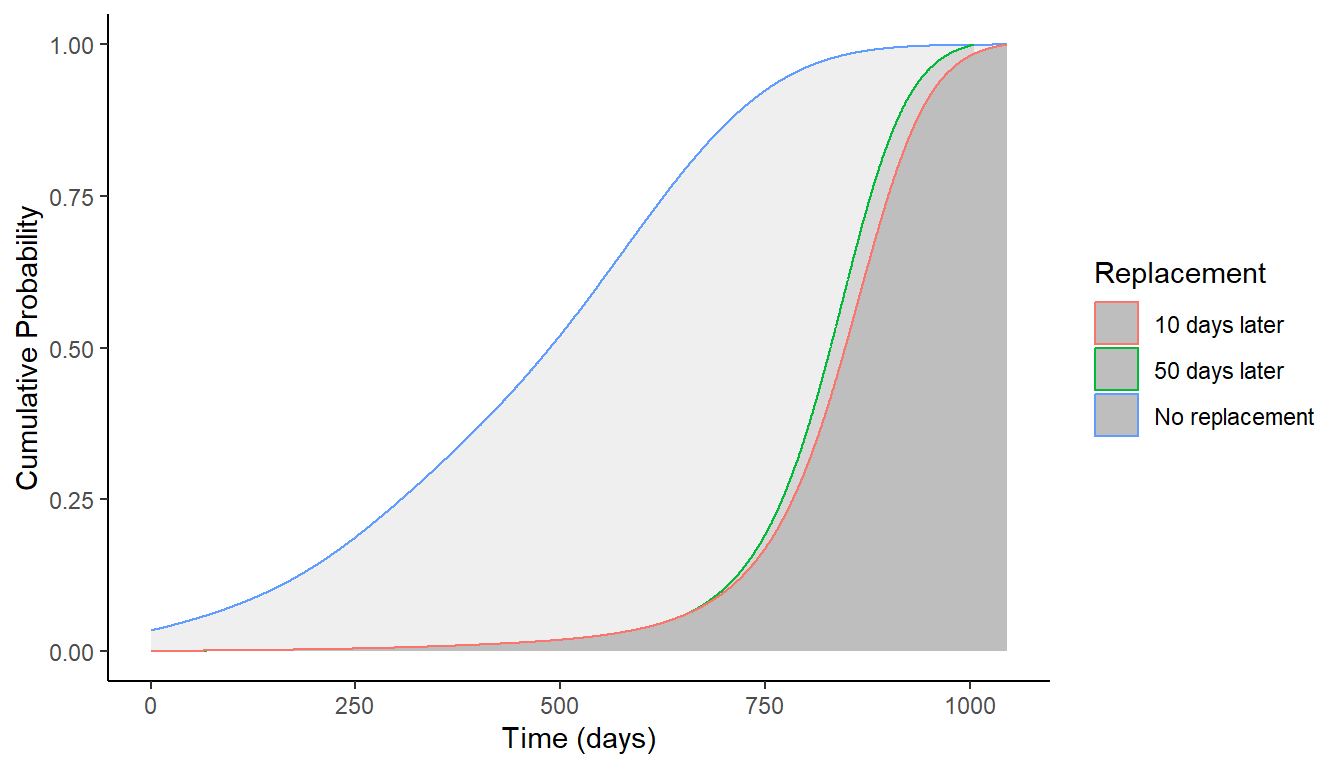
(#fig:img_cumulative)Figure 11. Renewal Rates

From this point on, the math for $z(t)$, $H(t)$, and $AFR(t)$ for renewal rates gets a little tricky, so we’ll save that for another day. But you’re well on your way to working with life distributions!

Function	Name	Formula	Equivalency	Meaning
\(F(t)\)	Failure Function	\(1 - e^{-\lambda t}\)	\(1 - e^{-H(t)}\)	Cumulative Distribution Function (CDF) of Lifespans
\(R(t)\)	Reliability Distribution	\(e^{-\lambda t}\)	\(e^{-H(t)}\)	Remainder of CDF for Lifespans
\(f(t)\)	Change in Failure Function	\(\frac{F(t + \Delta t) - F(t)}{\Delta t}\)	\(-R'(t)\)	Change in CDF at time \(t_{2}\) \(-\) at \(t_{1}\), per extra timestep
\(z(t)\)	Failure Rate (Hazard Rate)	\(\frac{f(t)}{R(t)}\)	\(\lambda = \frac{1}{m}\)	Mean Failure Rate \(\lambda\); Inverse of Mean Time to Fail \(m\)
\(H(t)\)	Accumulative Hazard Rate	\(-log( R(t) )\)	\(\lambda t\)	Total Risk of Failure gained from time 0 to \(t\)
\(AFR(t_1,t_2)\)	Average Failure Rate	\(\frac{H(t_{2}) - H(t_{1})}{t_{2} - t_{1}}\)	\(\frac{log(R(t_{1})) -log(R(t_{2})}{t_{2} - t_{1}}\)	Average failures per timestep between times \(t_{1}\) and \(t_{2}\)