Bundles of coloured filaments streaming across a dark ground
Week: Probability

Lesson 3: Probability Functions

Tools for Risk Analysis
Tim Fraser
Tim Fraser, PhD
Assistant Teaching Professor, Systems Engineering
Cornell University
SYSEN 5300: Systems Engineering & Six Sigma
for Design and Operation of Reliable Systems
Learning Outcomes
Target with arrow in the bullseye
  • Risk Analysis
    • Risk assessment and risk characterization
    • Failure Modes and Effects Analysis
    • Fault trees and event trees under uncertainty
  • Modeling Reliability
    • Component and system reliability
    • Physical acceleration models
    • Required function, stated conditions, specified time
    • One element of the broader risk analysis
Learning Outcomes
Target with arrow in the bullseye
  • Quality Control
    • Six sigma and statistical process control
    • Detect when performance is deteriorating
    • Take corrective action in time
  • System Improvement
    • Optimize system design for reliability
    • Design of experiments
    • Response surfaces — innovation, problem solving, and discovery

Today's Class

  1. Key Functions
  2. Probability Functions
  3. Probability Rules
  4. Functions [Demo]
  5. Appendix: Bayes Rule
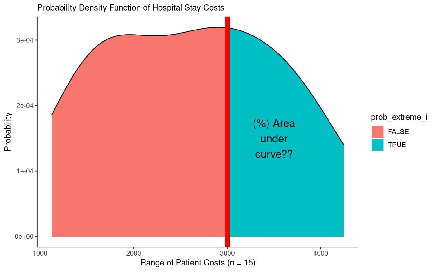
Probability density function of hospital stay costs, split at $3000 by a red line, the right tail labelled ‘(%) Area under curve??’
Investigate Distributions with Probability Functions
Key Functions (1)
New functions
library(dplyr)
library(ggplot2)
library(broom)
library(mosaicCalc)
  • bind_rows(): stacks 2 or more data.frames on top of each other, matching columns by name.
  • mutate(): creates or edits variables in a data.frame.
  • summarize(): consolidates many rows of data into a single summary statistic (or several).
  • tibble(): creates a data.frame, but fancy! Can reference other vectors within the tibble.
Key Functions (2)
Using mutate() and summarize()
Example data.frame
mycoffee
##       style price         shop
## 1     latte     5         <NA>
## 2 cappuccino    4         <NA>
## 3  americano    3         <NA>
## 4     coffee    3 Gimme Coffee
## 5 hot cocoa     2    Starbucks
mycoffee = mycoffee %>%
  mutate(purchased =
    c(5, 4, 10, 2, 1))
Key Functions (2)
Using mutate() and summarize()
mycoffee %>%
  # Summarize data.frame into one row
  summarize(
    # Calculate mean price of drinks
    mean_price = mean(price),
    # Calculate total drinks purchased
    total_purchased = sum(purchased))
##   mean_price total_purchased
## 1        3.4              22

Probability Functions


Lesson 3 — Using Probability Density Functions & Cumulative Density Functions
Probability Functions (1)
Probability Density Function
  • For a vector x, the probability density function is a curve providing the probability (y) of each value across the range of x.
  • It shows the relative frequency (probability) of each possible value in the range.
obs = c(1126, 1493, 1528, 1713, 1912, 2060, 2541, 2612,
        2888, 2915, 3166, 3552, 3692, 3695, 4248)
Probability Functions (1)
Probability Density Function (PDF)
Probability density function of hospital stay costs, split at $3000 by a red line, the right tail labelled ‘(%) Area under curve??’
Cumulative Distribution Function (CDF)
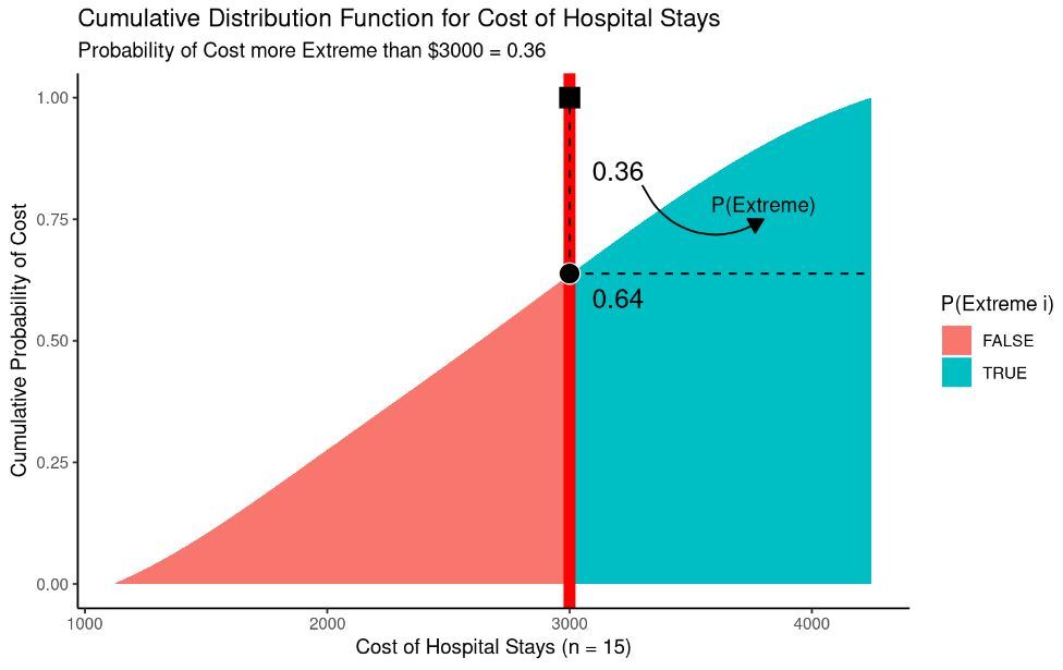
Cumulative distribution function for cost of hospital stays, rising to 1.00, annotated 0.36 above and 0.64 below a red line at $3000, with P(Extreme) marked
cumsum(prob) / sum(prob)  →  Probability of Cost more Extreme than $3000 = 0.36
Probability Functions (2)
Applying PDFs and CDFs

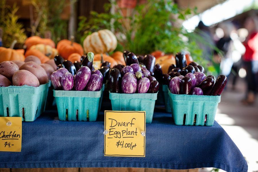
The Ithaca Farmers Market is a vendor-owned cooperative that runs a Saturday-and-Sunday morning market for produce and hand made goods on the Cayuga Lake waterfront. This Saturday, a volunteer tracked 500 customers and recorded how many stalls each customer visited.

The average customer visited…
Mean5.5 stalls
Median5 stalls
Standard deviation2.5 stalls
  • But their spreadsheet got blown away into the lake! Can we still estimate visitation patterns with these statistics?
Farmers market stall: pint baskets of purple dwarf eggplant and potatoes on a blue cloth with handwritten price signs
Probability Functions (3)
Simulating Unobserved Distributions

We don't have the actual data, but we know several basic features of our distribution!

  • Our variable is visits, a count ranging from 0 to infinity. (Can't have -5 visits, can't have 1.3 visits.)
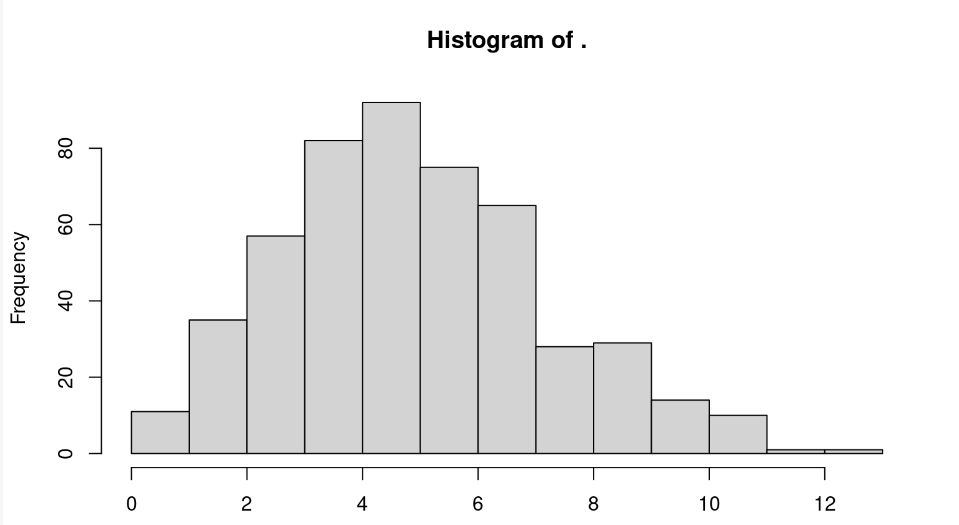
  • The median (5) is less than the mean (5.5), so our distribution is right-skewed.
# Randomly sample 500 visits from a
# poisson distribution with a mean of 5.5
visits = rpois(n = 500, lambda = 5.5)
# Check out the distribution!
visits %>% hist()
Histogram of simulated visits, peaking near 5 and tailing off past 10
Probability Functions (4)
Your Guide to Probability Estimation given Unobserved Distributions
Table 1: Probability Functions (r, d, p, and q)
Meaning · Purpose · Main Input · Normal · Poisson · Gamma · Exponential
Random Draws from Distribution · Simulate a distribution · n = # of simulations · rnorm() · rpois() · rgamma() · rexp()
Probability Density Function · Get Probability of Value in Distribution · x = value in distribution · dnorm() · dpois() · dgamma() · dexp()
Probability Functions (4)
Your Guide to Probability Estimation given Unobserved Distributions
Table 1: Probability Functions (r, d, p, and q)
Meaning · Purpose · Main Input · Normal · Poisson · Gamma · Exponential
Cumulative Distribution Function · Get % of Distribution LESS than Value · q = a cumulative probability · pnorm() · ppois() · pgamma() · pexp()
Quantiles Function · Get Value of any Percentile in Distribution · p = percentile · qnorm() · qpois() · qgamma() · qexp()
Probability Functions (5)
Finding probability densities
# Get the frequency for 5 visits
# in the distribution
pd5 = dpois(5, lambda = 5.5)
# Check it!
pd5
## [1] 0.1714007
If you don't have the raw data…
# Approximate the PDF of our
# simulated visits
dsim = visits %>% density() %>%
  approxfun()
# Try our density function for
# our simulated data!
dsim(5)
## [1] 0.1759108
If you do have the raw data….
Probability Functions (6)
Finding cumulative probabilities

What percentage of customers stopped by over 5 stalls?

# Get the cumulative frequency for a
# value (5) in the distribution
cd5 = ppois(q = 5, lambda = 5.5)
1 - cd5
## [1] 0.4710813
If you don't have the raw data…
Probability Functions (6)
Finding cumulative probabilities
psim = visits %>% density() %>% tidy() %>%
  # Get cumulative probability distribution
  arrange(x) %>%
  # Get cumulative probabilities
  mutate(y = cumsum(y) / sum(y)) %>%
  # Turn it into a literal function!
  approxfun()
If you do have the raw data….
# Check it!
psim(5)
## [1] 0.4642488
Probability Functions (6)
Finding quantiles

How many visits did people usually make? Estimate the interquartile range (25th-75th percentiles) of the unobserved distribution.

q5 = qpois(p = c(.25, .75), lambda = 5.5)
# Check it!
q5
## [1] 4 7
Looks like 50% of folks visited between 4 and 7 stalls
If you don't have the raw data…
Probability Functions (6)
Finding quantiles
qsim = tibble(
  # Get a vector of percentiles from 0 to 1, i
  x = seq(0, 1, by = 0.001),
  # Using our simulated distribution,
  # get the quantiles (values) at those points
  y = visits %>% quantile(probs = x)) %>%
  # Approximate function!
  approxfun()
If you do have the raw data….
# Check it!
qsim(c(.25, .75))
## [1] 4 7
Learning Check
Farmers market stall: pint baskets of purple dwarf eggplant and potatoes on a blue cloth with handwritten price signs

What if we are not certain whether our unobserved vector of visits has a Poisson distribution or not? Please calculate the probability that customers will stop at more than 5 stalls, using the Normal & Exponential distributions.

Out of n = 500 customers, the average customer visited a mean of 5.5 stalls and a median of 5 stalls, with a standard deviation of 2.5 stalls.

Probability · Live Lab
BREAK TIME
Grogu (Baby Yoda) cradling a cup of soup in both hands

Probability Rules


Lesson 3 — Conditional Probability & Total Probability
Probability Rules (1)
Conditional Probability
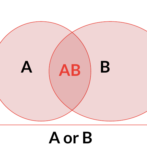
Two overlapping pink circles labelled A and B, their intersection labelled AB, with a bracket beneath labelled ‘A or B’
Conditional Probability: probability of two events happening together reflects the probability of the first happening, times the probability of the second happening given that the first has already occurred.
P(A)0.25Area of A
P(B)0.50Area of B
P(B | A)0.2% of A that is B
P(AB)0.05Area of AB
P(A or B)0.7P(A) + P(B) - P(AB)

P(AB) = P(A) x P(B|A)  →  0.05 = 0.25 x 0.2

Probability Rules (2)
Visual Conditional Probability
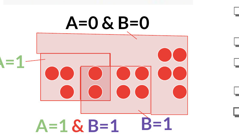
P(AB) = P(A) × P(B|A)
Overlapping outlined regions of red dots: the whole set labelled A=0 & B=0, a left box labelled A=1, a right box labelled B=1, and their overlap labelled A=1 & B=1
P(A=1)5 / 14
P(B=1)6 / 14
P(A=0&B=0)5/ 14
P(A=1 or B=1)9/14
P(B=1|A=1)2/5
P(A=1&B=1)2/14

2/14 = 5/14 * 2/5

Probability Rules (3)
Total Probability
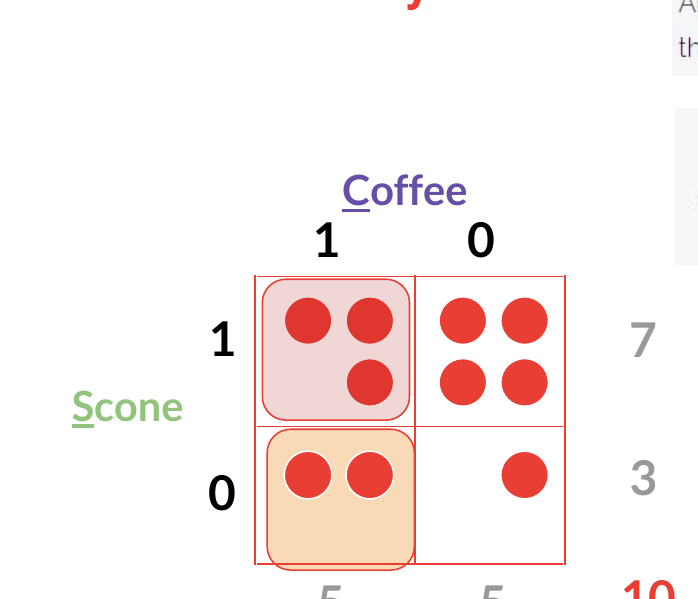
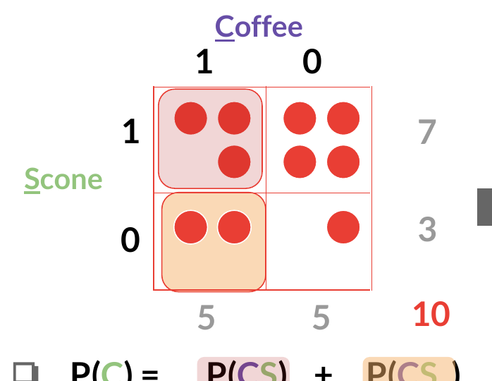
A two-by-two grid of red dots cross-tabulating Scone (1, 0) against Coffee (1, 0), with margins 7, 3, 5, 5 and a total of 10
Any event A that is mutually exclusive from event E (can't happen at the same time) has the following probability..

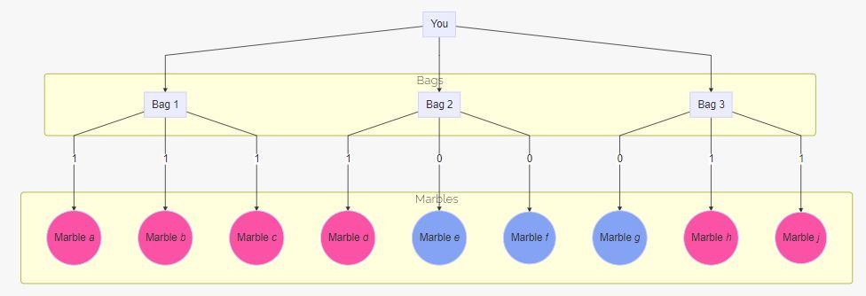
P(A) = ∑i=1n P(A|Ei) × P(Ei)

A probability tree branching from one node into three bags, each into several marbles

P(C) = P(CS) + P(CS0)

Total Probability · Bags & Marbles

Functions [Demo]


Lesson 3 — How to make a function in R/Python

Further Reference


Probability Rules — The following slides give extra details that may help, if relevant to your projects.
A corgi in a red cape, standing on its hind legs and looking up
Probability Rules
Bayes Rule
A steaming white cup of coffee on a saucer on a wooden cafe table

A local coffee chain needs your help to analyze their supply chain issues. They know that their scones help them sell coffee, but does their coffee help them sell scones?

  • Over the last week, when 7 customers bought scones, 3 went on to buy coffee.
  • When 3 customers didn't buy scones, just 2 bought coffee.
  • In general, 7 out of 10 of customers ever bought scones.
  • What's the probability that a customer will buy a scone, given that they just bought coffee?
Bayes Rule (Visually)
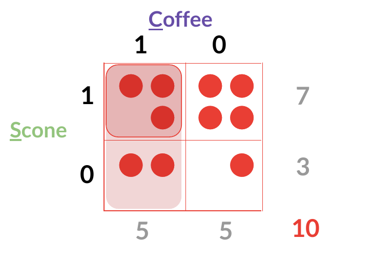
Two-by-two grid of red dots cross-tabulating Scone against Coffee, with the Coffee=1 column shaded, margins 7, 3, 5, 5 and a total of 10

Can we deduce P(Scone | Coffee) on our own?

P(Scone=1)7 / 10
P(Coffee=1)5 / 10
P(Scone=0)3 / 10
P(Coffee=0)5 / 10
P(Scone=1 | Coffee=1)3 / 5
P(Coffee=1 | Scone=1)3 / 7
P(Scone=1 | Coffee=0)2 / 5
P(Coffee=0| Scone=1)4 / 7
Bayes Rule (Visually)
Two-by-two grid of red dots cross-tabulating Scone against Coffee, with the Coffee=1 column shaded, margins 7, 3, 5, 5 and a total of 10
  • P(S|C) = P(C|S)   x   P(S)   /   P(C)
  • 3/5 = 3 / 7   x   7/10   /   5 /10
P(Scone=1)7 / 10
P(Coffee=1)5 / 10
P(Scone=0)3 / 10
P(Coffee=0)5 / 10
P(Scone=1 | Coffee=1)3 / 5
P(Coffee=1 | Scone=1)3 / 7
P(Scone=1 | Coffee=0)2 / 5
P(Coffee=0| Scone=1)4 / 7
Bayes Rule (Visually)
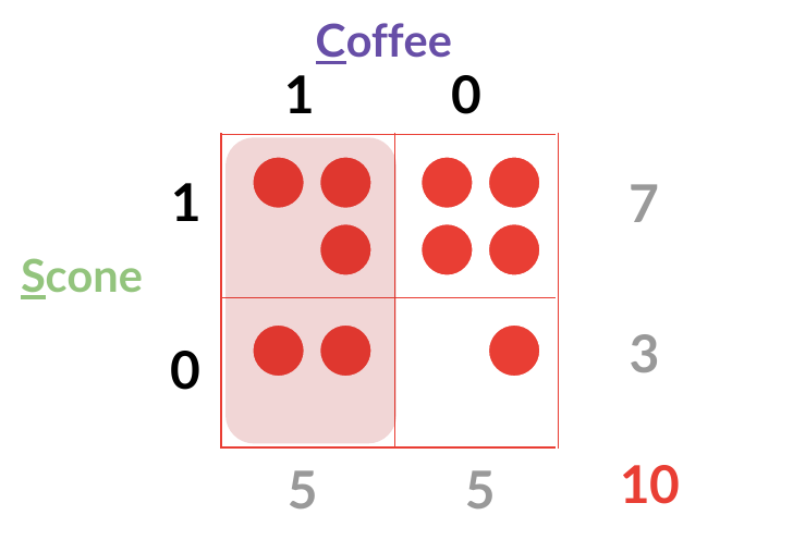
The same Scone-by-Coffee dot grid with the Coffee=1 column shaded a flat pink

But what if we don't know P(Coffee)?

P(Scone=1)7 / 10
P(Coffee=1)5 / 10
P(Scone=0)3 / 10
P(Coffee=0)5 / 10
P(Scone=1 | Coffee=1)3 / 5
P(Coffee=1 | Scone=1)3 / 7
P(Scone=1 | Coffee=0)2 / 5
P(Coffee=0| Scone=1)4 / 7
Bayes Rule (Visually)
Scone-by-Coffee dot grid with the Scone=1 cell shaded pink and the Scone=0 cell shaded tan
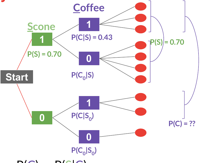
  • P(C) = P(CS) + P(CS0)
  • P(CS) = P(S) x P(C|S) = P(C) x P(S|C)
  • P(CS0) = P(S0) x P(C|S0) = P(C) x P(S0|C)
Probability tree from Start to Scone 1/0 to Coffee 1/0, each ending in red dots, annotated P(S) = 0.70, P(C|S) = 0.43 and P(C) = ??
Bayes Rule (Visually)
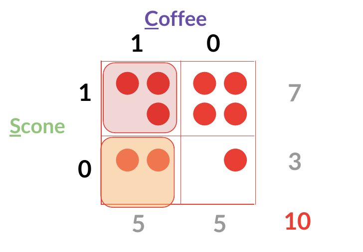
Scone-by-Coffee dot grid with the Scone=0 & Coffee=1 cell shaded tan and its dots drawn in orange
  • P(C) = P(S) x P(C|S) + P(S0) x P(C|S0)
  • 5/10 = 7/10 x 3/7   +   3/10 x 2/3
P(Scone=1)7 / 10
P(Coffee=1)5 / 10
P(Scone=0)3 / 10
P(Coffee=0)5 / 10
P(Scone=1 | Coffee=1)3 / 5
P(Coffee=1 | Scone=1)3 / 7
P(Coffee=1| Scone=0)2 / 3
Bayes Rule (Formal Statement)

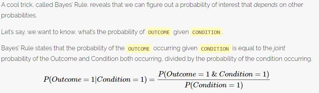
Bayes' Rule states that the probability of the OUTCOME occurring given CONDITION is equal to the joint probability of the Outcome and Condition both occurring, divided by the probability of the condition occurring.

P(Outcome = 1 | Condition = 1) equals P(Outcome = 1 & Condition = 1) divided by P(Condition = 1)