32 Appendix: tidyfault for Fault Tree Analysis
Getting Started
Fault trees are visual representation of boolean probability equations, typically depicting the sets of necessary events leading to system failure. We learned about them earlier in the textbook, but you might be wondering, with all your ggplot skills now, can you visualize a fault tree in ggplot? And are there other technical solutions for computing fault tree quantities of interest?
Good news! There is! This tutorial will explain how to use the tidyfault package to work with fault trees.
32.1 Visualizing Fault Trees in R
We can draw fault trees easily enough by hand, but how do we record their data in a machine readable format? We can use conventions from network science to record these data in two lists: (1) an ‘edgelist’ of edges connecting nodes, and (2) a ‘nodelist’ of nodes, connected by edges.
32.1.1 Making a Nodelist
We can use the tribble() function available when loading the tidyverse package to write out small data.frames row by row. In nodes, our nodelist:
every node must have a unique ID, called
name.some events reappear multiple times in the same tree; we must give these nodes different
namebut the sameeventname.each node should be classified by
typeas (1) anandgate, (2) anorgate, or (3)nota gate. We can usefactor()to tell R to always remember"and","or", and"not"in that order (useful forggplotlegends).classic fault trees sometimes write events and the gates that condition them as separate nodes, but as far as the graph is concerned, they are really the same node. So, remember to combine them for analysis.
# Let's make a data.frame of nodes!
tribble(
  # Make the headers, using a tilde
  ~id, ~event, ~type,
  # Add the value entries
  "T",   "T",   "top",
  "G1",  "G1",  "and",
  # Notice how event 'B' appears twice,
  # so it has a logical but differentiated `name` "B1" and "B2"?
  "B1",  "B",   "not",
  "B2",  "B",   "not",
  "C1",  "C",   "not") %>%
  # Classify 'type' as a factor, with specific levels
  mutate(type = factor(type, levels = c("top", "and", "or", "not")))
## # A tibble: 5 × 3
## id event type
## <chr> <chr> <fct>
## 1 T T top
## 2 G1 G1 and
## 3 B1 B not
## 4 B2 B not
## 5 C1 C not
32.1.2 Making an Edgelist
Next, we can use tribble() to make an edgelist of our fault tree (or use read_csv() to read in an edgelist). Edgelists should follow these conventions:
- each row shows a unique edge between nodes, recording their node
ids from the top-down in thefromandtocolumns.
## # A tibble: 4 × 2
##   from  to
##   <chr> <chr>
## 1 T     G1
## 2 G1    G2
## 3 G2    B1
## 4 G2    G5
32.2 Our Data
In this example, we’re going to use the default data in tidyfault, called fakenodes and fakeedges. You can download it like this:
## # A tibble: 12 × 3
##       id event type
##    <dbl> <chr> <fct>
##  1     1 T     top
##  2     2 G1    and
##  3     3 G2    and
##  4     4 G3    or
##  5     5 G4    and
##  6     6 G5    or
##  7     7 A     not
##  8     8 B     not
##  9     9 B     not
## 10    10 C     not
## 11    11 C     not
## 12 12 D not## # A tibble: 11 × 2
## from to
## <dbl> <dbl>
## 1 1 2
## 2 2 3
## 3 3 8
## 4 3 6
## 5 6 10
## 6 6 12
## 7 2 4
## 8 4 7
## 9 4 5
## 10 5 9
## 11 5 11
32.3 Getting a Fault Tree Layout
Using tidyfault‘s illustrate() function, we can quickly assign x and y coordinates for a ’tree’ layout to to our fakenodes and fakeedges. We say type = "both" because we want to receive coordinates for both the nodes and edges.
This returns a list() object. list() objects are collections of data.frames - sort of like a vector whose values are entire data.frames. We can query the values inside lists by using the $, just like a data.frame.
##    x y id event type
## 1  0 4  1     T  top
## 2  0 3  2    G1  and
## 3 -1 2 3 G2 and## # A tibble: 3 × 5
## # Groups: edge_id [2]
## edge_id direction id x y
## <int> <chr> <dbl> <dbl> <dbl>
## 1 1 from 1 0 4
## 2 1 to 2 0 3
## 3 2 from 2 0 332.4 Visualize a Fault Tree
ggplot() +
  # Plot each line corresponding to the unique edge id, used to group them
  geom_line(data = gg$edges, mapping = aes(x = x, y = y, group = edge_id)) +
  # Plot each point
  geom_point(data = gg$nodes,
             mapping = aes(x = x, y = y, shape = type, fill = type),
             size = 10) +
  # Plot labels!
  geom_text(data = gg$nodes, mapping = aes(x = x, y = y, label = event)) +
  # We can also assign shapes!
  # (shapes 21, 22, 23, 24, and 25 have fill and color)
  scale_shape_manual(values = c(22, 24, 25, 21)) +
  # And assign some poppy colors here
  scale_fill_manual(values = c("darkgrey", "cyan", "coral", "lightgrey")) +
  # Finally, we can make a clean void theme, with the legend below.
  theme_void(base_size = 14) +
  theme(legend.position = "bottom")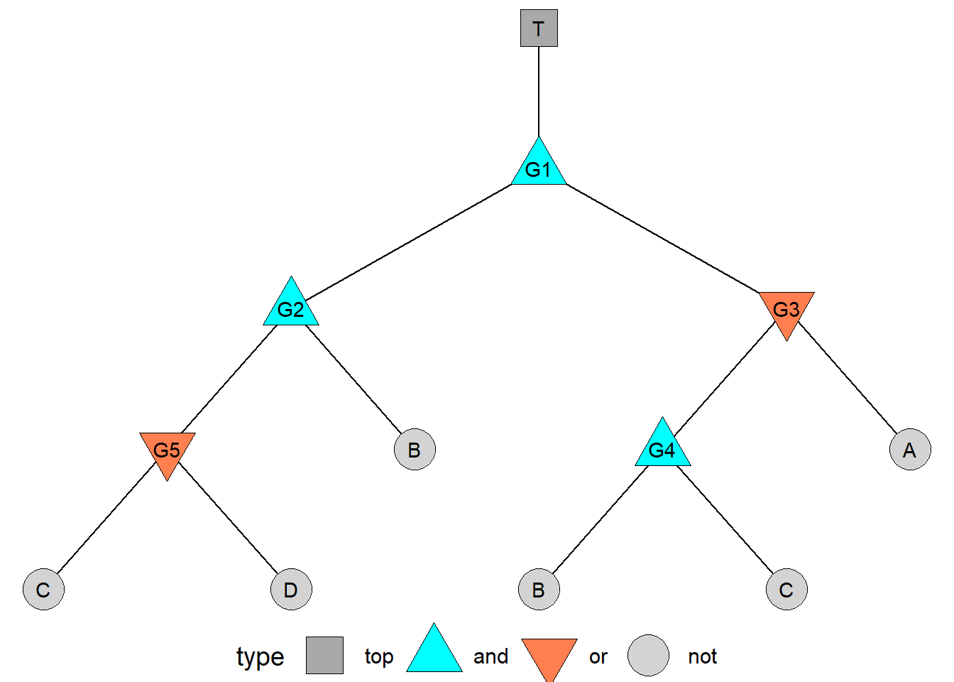
32.5 Cutsets
Fault Trees are big - and some events are more critical than others. We want to identify two kinds of information.
cutsets: all the possible sets of events which together trigger failure, called cutsets.
minimal cutsets: the most reduced set of events which trigger failure.
To do this, we’re going to use an algorithm, called the MOCUS top-down algorithm. I wrote it in R for you! Yay!
32.6 Gates
## # A tibble: 6 × 6
##   gate  type  class     n set           items
##   <chr> <fct> <fct> <int> <chr>         <list>
## 1 T     top   top       1 " (G1) "      <chr [1]>
## 2 G1    and   gate      2 " (G2 * G3) " <chr [2]>
## 3 G2    and   gate      2 " (B * G5) "  <chr [2]>
## 4 G3    or    gate      2 " (A + G4) "  <chr [2]>
## 5 G4    and   gate      2 " (B * C) "   <chr [2]>
## 6 G5    or    gate      2 " (C + D) "   <chr [2]>
32.7 Equations
To get the full boolean equation of the fault tree, use equate()!
## [1] " ( ( (B * (C + D) ) * (A + (B * C) ) ) ) "We can format it as a function too!
f = g %>% equate() %>% formulate()

# Suppose there is each of these probabilities that A, B, C, and D occur
# what's the probability of the top event?
f(A = 0.3, B = 0.5, C = 0.1, D = 0.5)
## [1] 0.10532.8 Minimal Cutsets
To simplify down to the minimal cutsets, use concentrate()! It’s pretty quick for small graphs, but gets exponentially longer the more nodes you add. (Especially with OR statements.) That’s MOCUS’s value as well as its tradeoff.
## [1] "B*C" "A*B*D"32.9 Coverage
We might want to know, how important are each of my minimal cutsets? We can compute the total number of cutsets that include the minimal cutset, the total cutsets leading to failure in general, and the percentage (coverage) of cutsets containing your minimal cutset out of all total cutsets leading to failure. It’s basically a measure of the explanatory power of your cutsets!
## # A tibble: 2 × 5
##   mincut query                                        cutsets failures coverage
##   <chr>  <chr>                                          <int>    <int>    <dbl>
## 1 A*B*D  filter(A == 1, B == 1, D == 1, outcome == 1)       2        5      0.4
## 2 B*C    filter(B == 1, C == 1, outcome == 1)               4        5      0.8