23 Appendix: Using `fitdistr` to Fitting Distribution Parameters

This tutorial will introduce you to **Fitting Distribution Parameters in R, teaching you how to use the fitdistr() function from the MASS package in R.

This training continues on our previous work on Descriptive Statistics. Often, we might want to approximate statistics describing the shape of distributions, but there may not be a clear analytical method (eg. method of moments) to do so. We can use the power of optimization to help us instead, using a brute-force method to find the value most likely to be the statistic that actually fits our distribution. We can ask R to compute the values of those statistics using the MASS package’s fitdistr().

Getting Started

Please open up your project on Posit.Cloud, for our Github class repository. Start a new R script (File >> New >> R Script). Save the R script as appendix_fitdistr.R. And let’s get started!

Load Packages

# Load dplyr, which contains most data wrangling functions
library(dplyr)
# Load the fitdistr() function directly from the MASS package. 
# We'll do this, rather than loading the whole MASS package, because MASS will cancel out some dplyr functions that share the same names otherwise. See how fitdistr has now shown up in your environment as a function?
fitdistr = MASS::fitdistr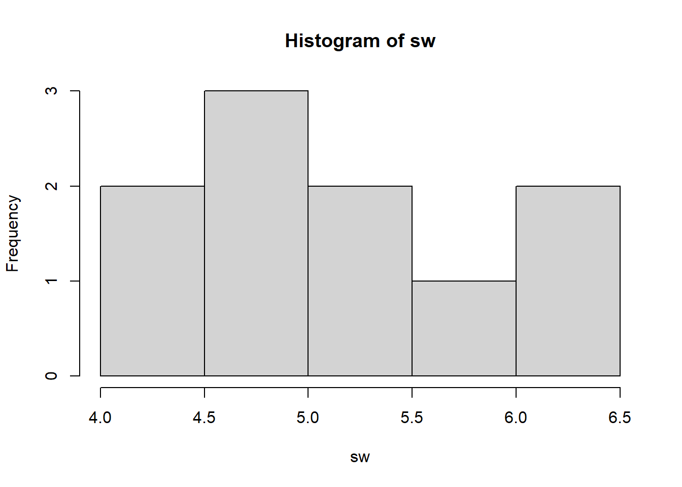

23.0.1 Our Data

As our raw data, let’s use our vector of seawall heights sw. Its raw distribution can be visualized with hist(sw).

# Let's remake again our vector of seawall heights
sw <- c(4.5, 5, 5.5, 5, 5.5, 6.5, 6.5, 6, 5, 4)
hist(sw)

23.1 Example: Exponential Distribution

We have our vector of seawall heights sw. We have 2 main ways of calculating statistics that describe the distribution of sw. These include an analytical approach (method of moments) and a brute-force approach (maximum likelihood estimation).

In the analytical approach (method of moments), which we learned in the main textbook, we use formula that have been derived by mathematicians to describe the parameters of a particular distribution.
In the brute-force approach (maximum likelihood estimation), we use a secondary parameter called likelihood to find the parameter values most likely to fit your data. We say, if the parameter had value A (for example), what’s the joint probability (likelihood) of finding your observed values (sw) in a distribution with that trait A? We use maximum likelihood estimation to iteratively test various different values for parameter A, and choose the value that provides the highest likelihood - a.k.a. the maximum likelihood.

Note: Remember: a parameter is a single number that describes a full population. A statistic is a single number that describes a sample. This key difference aside, the terms are largely interchangeable.

Let’s use the exponential distribution as a helpful example. It has one parameter - rate (also known as \(\lambda\)), describing \(\frac{1}{ mean }\).

Let’s calculate the rate parameter a few ways, using (1) the method of moments, (2) maximum likelihood estimation (MLE) using fitdistr(), and (3) maximum likelihood estimation (MLE) using optim().

23.2 Method of Moments

# Let's use the method of moments to find the inverse mean
1 / (sum(sw) / length(sw))

## [1] 0.1869159

# Equivalent to...
1 / mean(sw)

## [1] 0.1869159

23.3 MLE with `fitdistr()`

Let’s ask fitdistr to run maximum likelihood estimation.

Maximum likelihood estimation requires a benchmark distribution to compare against, so we need to specify the distribution type as densfun = [type name]. In this case, let’s do exponential. (See a list of supported distributions using ?MASS::fitdistr)

sw %>% MASS::fitdistr(densfun = "exponential")

##       rate   
##   0.18691589 
##  (0.05910799)

Pretty darn similar to the value we got from the method of moments, right?

23.4 MLE with `optim()`

Alternatively, we could run maximum likelihood estimation manually, using optim(). optim() is R’s built in optimization function. We’ll learn maximum likelihood estimation a little more later in the book. The key idea is this:

dexp(x = 2, rate = 0.1) gives the probability of the value x = 2 showing up in an exponential distribution characterized by a parameter rate = 0.1.

dexp(x = 2, rate = 0.1)

## [1] 0.08187308

dexp(x = sw, rate = 0.1) gives the probabilities for each value of x if they showed up in an exponential distribution characterized by a parameter rate = 0.1.

# You can also pipe the values of x into dexp() like this
sw %>% dexp(rate = 0.1)

##  [1] 0.06376282 0.06065307 0.05769498 0.06065307 0.05769498 0.05220458
##  [7] 0.05220458 0.05488116 0.06065307 0.06703200

The joint probability of these values of x occurring together is called the likelihood. We can take the product using prod().

# Let's get the likelihood of these values...
sw %>% dexp(rate = 0.1) %>% prod()

## [1] 4.748151e-13

Likelihood tend to be very small numbers, so a helpful trick is to calculate the log-likelihood instead, meaning the sum of logged probabilities.

# See how these two processes produce the same output?
# Get the log of probabilities multiplied together...
sw %>% dexp(rate = 0.1) %>% prod() %>% log()

## [1] -28.37585

# Get the sum of logged probabilities...
sw %>% dexp(rate = 0.1) %>% log() %>% sum()

## [1] -28.37585

# They're equivalent

Then, we write up a short function called loglikelihood(), including two inputs (1) par and (2) our data x. I added an example value 0.1 to par just as a reminder for what it means.

loglikelihood = function(par = 0.1, x){ dexp(x = x, rate = par) %>% log() %>% sum()   }
# Try it!
loglikelihood(par = 0.1, x = sw)

## [1] -28.37585

Finally, we run an optimizer using optim(), supplying a starting value for search par = 0.1, our raw data x, and our function loglikelihood. We want to maximize the loglikelihood, but optim() minimizes by default, so we’ll say, control = list(fnscale = -1) to flip the scale.

optim(par = c(0.1), x = sw, fn = loglikelihood, control = list(fnscale = -1))

## $par
## [1] 0.1869531
## 
## $value
## [1] -26.77097
## 
## $counts
## function gradient 
##       24       NA 
## 
## $convergence
## [1] 0
## 
## $message
## NULL

Compare the final parameter value against fitdistr’s results! They’re about the same.

fitdistr(x = sw, densfun = "exponential")

##       rate   
##   0.18691589 
##  (0.05910799)

Voila! You made your own maximum likelihood estimator manually. Certainly, optim() was a little more time consuming, but now you know how fitdistr truly works inside!

23.5 Applications

Let’s try applying the same general approach with fitdistr to other distributions.

23.5.1 Normal Distribution

What parameter values would best describe our distribution’s shape, if this data were from a normal distribution? Remember, normal distributions have a mean and a sd.

# Method of Moments
sw %>% mean()

## [1] 5.35

sw %>% sd()

## [1] 0.8181958

# Maximum Likelihood Estimation
sw %>% fitdistr(densfun = "normal")

##      mean         sd    
##   5.3500000   0.7762087 
##  (0.2454588) (0.1735655)

23.5.2 Poisson Distribution

What parameter values would best describe our distribution’s shape, if this data were from a Poisson distribution? Remember, poisson distributions have a lambda parameter describing the mean.

# Method of moments
sw %>% mean()

## [1] 5.35

# Maximum Likelihood Estimation
sw %>% fitdistr(densfun = "poisson")

##     lambda  
##   5.3500000 
##  (0.7314369)

23.5.3 Gamma Distribution

What parameter values would best describe our distribution’s shape, if this data were from a Gamma distribution? Remember, gamma distributions have a shape parameter ` \(\approx \frac{mean^{2}}{ variance}\) and a scale parameter \(\approx \frac{variance}{ mean }\).

# Method of Moments
# For shape, we want the rate of how much greater the mean-squared is than the variance.
mean(sw)^2 / var(sw)

## [1] 42.7556

# For rate, we like to get the inverse of the variance divided by the mean.
1 / (var(sw) / mean(sw) )

## [1] 7.991701

# Maximum Likelihood Estimation
sw %>% fitdistr(densfun = "gamma")

##      shape       rate   
##   46.711924    8.731202 
##  (20.815512) ( 3.911664)

23.5.4 Weibull Distribution

What parameter values would best describe our distribution’s shape, if this data were from a Weibull distribution? Remember, gamma distributions have a shape parameter and a scale parameter. (But we can’t easily use the method of moments here right now.)

# Estimate the shape and scale parameters for a weibull distribution
sw %>% fitdistr(densfun = "weibull")

##      shape       scale  
##   7.7312532   5.6881102 
##  (1.9038045) (0.2461222)

Learning Check 1

Question

You’ve been recruited to evaluate the frequency of Corgi sightings in the Ithaca Downtown. A sample of 10 students each reported the number of corgis they saw last Tuesday in town. Calculate the statistics summarizing each distribution, if it were a normal, poisson, exponential, gamma, or weibull distribution. Please use fitdistr for all your calculations.

Beth saw 5, Javier saw 1, June saw 10(!), Tim saw 3, Melanie saw 4, Mohammad saw 3, Jenny say 6, Yosuke saw 4, Jimena saw 5, and David saw 2.

[View Answer!]

First, let’s make the data.

# Make distribution of Corgis
corgi <- c(5, 1, 10, 3, 4, 3, 6, 4, 5, 2)

Next, let’s compute the estimated statistics using maximum likelihood estimation.

# Compute statistics for each distributions
corgi %>% fitdistr(densfun = "normal")

##      mean         sd    
##   4.3000000   2.3685439 
##  (0.7489993) (0.5296225)

corgi %>% fitdistr(densfun = "poisson")

##     lambda  
##   4.3000000 
##  (0.6557439)

corgi %>% fitdistr(densfun = "exponential")

##       rate   
##   0.23255814 
##  (0.07354134)

corgi %>% fitdistr(densfun = "gamma")

##      shape       rate   
##   3.2628624   0.7588054 
##  (1.3910572) (0.3497135)

corgi %>% fitdistr(densfun = "weibull")

##      shape       scale  
##   1.9207427   4.8617234 
##  (0.4566410) (0.8459497)

23.6 Conclusion

Congratulations! You now know how to use fitdistr() to approximate the parameters for a dataset, assuming various different types of distributions. You also learned maximum likelihood estimation, the core technique underneath fitdistr(), and how to perform it manually using optim(). Great work!

23 Appendix: Using fitdistr to Fitting Distribution Parameters