19 Useful Life Distributions (Exponential)
In this workshop, we’re going to learn some R functions for working with common life distributions, namely the Exponential distributions.
19.1 Getting Started
19.1.1 Load Packages
Let’s start by loading the tidyverse package, which will let us mutate(), filter(), and summarize() data quickly. We’ll also load mosaicCalc, for taking derivatives and integrals (eg. D() and antiD()).
19.1.2 Key Concepts
In this lesson, we’ll be building on several key concepts from prior lessons. I’ve defined them below as a helpful review.
life distribution: the distribution of a vector of \(n\) products, whose values recording the amount of time it took for each product to fail. In other words, its lifespan.
probability density function (PDF): the function describing the probability (relative frequency) of any value in a distribution.
cumulative distribution function (CDF): the function describing the cumulative probability of each successive value in a distribution. Spans from 0 to 1.
Have questions? I strongly recommend you review Workshops 2, 3, and 4 before this one! It will help it all fit together!
19.1.3 Our Data
In this workshop, we’re going to work with a data.frame called masks. An extremely annoying moment in the COVID-era is when a part of your mask snaps, requiring you to get a fresh mask. Let’s examine a (hypothetical) sample of n = 50 masks produced by Company X to explore how often this happens!
Please import the masks.csv data.frame below. Each row is a mask, with its own unique id. Columns describe how many hours it took for the left_earloop to snap, the right_earloop to snap, the nose wire to snap, and the fabric of the mask to tear.
## Rows: 50
## Columns: 5
## $ id            <dbl> 1, 2, 3, 4, 5, 6, 7, 8, 9, 10, 11, 12, 13, 14, 15, 16, 1…
## $ left_earloop  <dbl> 6, 16, 46, 4, 1, 5, 32, 35, 27, 3, 4, 7, 1, 20, 22, 17, …
## $ right_earloop <dbl> 12, 1, 17, 14, 19, 8, 18, 14, 5, 8, 8, 2, 12, 7, 20, 4, …
## $ wire          <dbl> 4, 1, 8, 29, 23, 8, 10, 38, 11, 31, 7, 4, 3, 33, 13, 2, …
## $ fabric        <dbl> 177, 462, 65, 405, 2483, 1064, 287, 2819, 1072, 288, 863…
19.2 Quantities of Interest
When we work with life distributions, we often want to find several useful quantities of interest (a.k.a. parameters) about them. Let’s find out how to do that with an exponential distribution!
19.2.1 Lack of Memory
Exponential distributions are famous for a key trait. The failure rate $ $ remains constant in an exponential distribution. The probability that a product fails in the next hour of use is the same at t = 0, t = 100, or t = infinity! It doesn’t worsen with time. (It’s the literal meaning of the saying, “if it is not broke, don’t fix it!”)
19.2.2 Mean Time to Fail
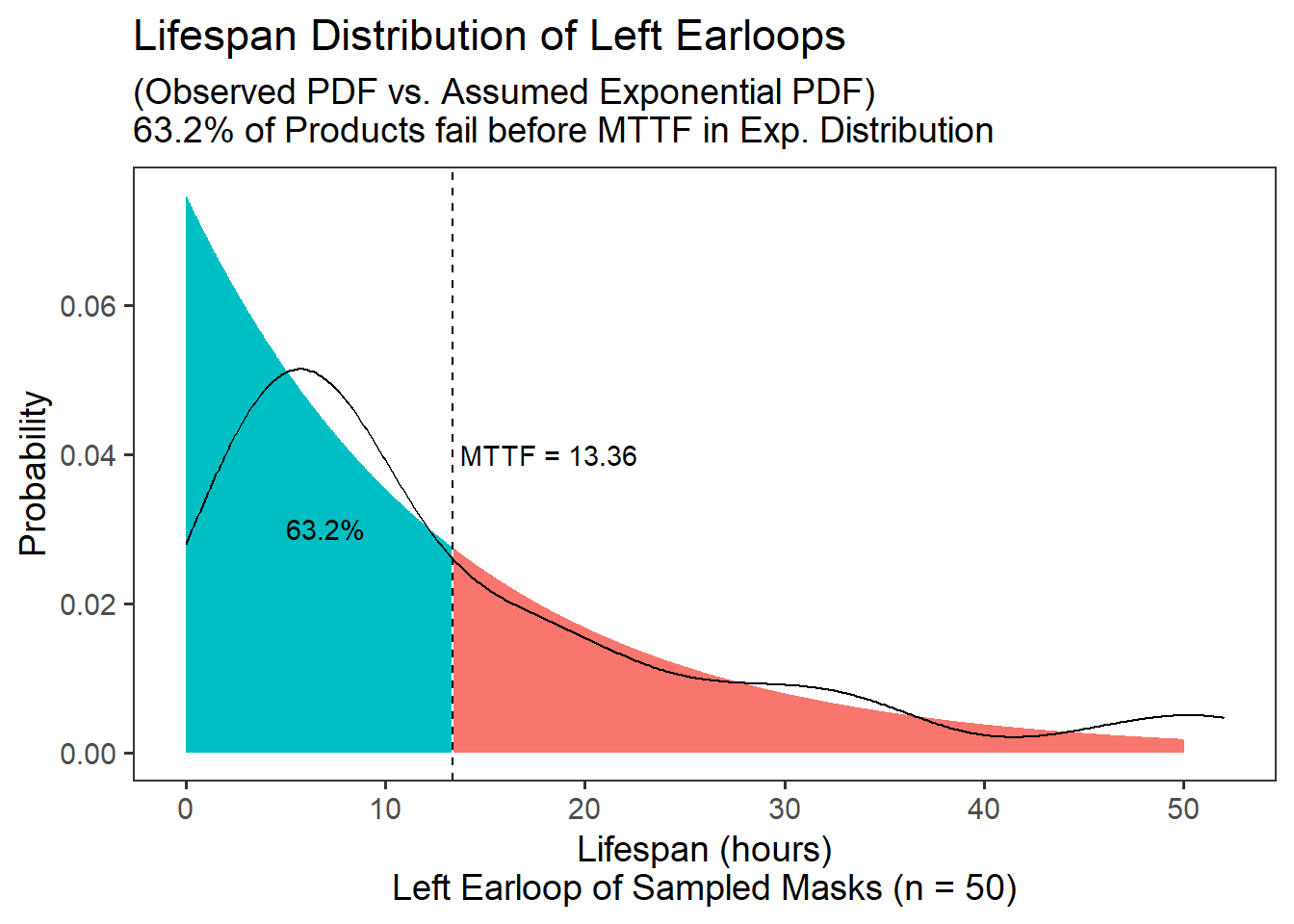
The Mean Time to Fail describes the mean of a lifespan distribution. For example, let’s calculate the mean time to fail (in hours) for a mask’s left_earloop in our sample.
stat <- masks %>%
  summarize(
    # We can take the mean of this vector of time to fail in hours
    mttf = mean(left_earloop),
    # Lambda is the reciprocal of the MTTF
    lambda = 1 / mttf)

# Check out the contents!
stat
## # A tibble: 1 × 2
## mttf lambda
## <dbl> <dbl>
## 1 13.4 0.0749In an exponential distribution, the MTTF always has a cumulative probability of 1 - 1 / e = 0.632. (This can be coded in R like so:)
## [1] 0.6321206Let’s assume our sample’s left earloops have an exponential lifespan distribution, and use pexp() to calculate the cumulative probability of getting an MTTF of 13.36. We’ll need to supply pexp() the benchmark in the distribution in question (mttf), plus the the rate parameter \(\lambda\), which we always need when simulating an exponential distribution.
## [1] 0.6321206Indeed, the figure below compares the observed PDF function (made using density()) to the assumed exponential PDF (made using dexp()), and we can see that that 63% of the distribution has failed by the Mean Time to Fail.
19.2.3 Mean Time to Fail via Integration
Mean Time to Fail (MTTF) can be number-crunched empirically as the mean of observed lifespans, assuming an exponential distribution. But it is also equal to the integral of the reliability function: $MTTF = _{0}^{}{R(t)dx} $.
So, let’s make ourselves a nice reliability function to help us calculate the MTTF.
We know the reliability function can be stated as \(R(t) = 1 - F(t)\).
Assuming an exponential distribution, the failure rate \(F(t) = 1 - e^{-\lambda t}\).
We know \(\lambda = \frac{1}{MTTF}\), and above, we found that lambda = 0.0748502994011976 for a left-earloop.
We can calculate it below…
# Use mosaicCalc's antiD function
# To get integral of r(t, lambda) as x goes from 0 to infinity
mttf = antiD(tilde = r(t, lambda) ~ t)
Great! We have developed our own mttf function for an exponential distribution! If we feed t a suitably large value, like 1000 (approaching infinity), we will reach the original observed/estimated mttf.
## [1] 13.36## [1] 13.36This only helps you if you know lambda, the inverse of the MTTF, or have the reliability function but not the MTTF.
19.2.4 Median Time to Fail \(T_{50}\)
We might also want to know the median time to failure (\(T_{50}\)), the value on the x axis that splits the area under the curve in half at 50% and 50%. We can calculate this as…
\(F(T_{50}) = 50\% = 0.5 = 1 - e^{-\lambda T_{50}}\)
where:
\(T_{50} = \frac{log(2)}{ \lambda } = \frac{0.693}{\lambda}\)
# Let's update stat to include the observed 'median'
# and 't50', the median assuming an exponential distribution

stat <- masks %>%
  summarize(
    # The literal mean time to fail
    # in our observed distribution is this
    mttf = mean(left_earloop),
    # And lambda is this...
    lambda = 1 / mttf,
    # The observed median is this....
    median = median(left_earloop),
    # But if we assume it's an exponential distribution
    # and calculate the median from lambda,
    # we get t50, which is very close.
    t50 = log(2) / lambda)

# Check it out!
stat
## # A tibble: 1 × 4
## mttf lambda median t50
## <dbl> <dbl> <dbl> <dbl>
## 1 13.4 0.0749 8 9.2619.2.5 Modal Time to Fail
Finally, the modal time to fail is pretty easy to calculate. Its the most common time to fail, also known as the max probability in a PDF.
masks %>%
  summarize(
    # Let's get lambda, the reciprocal of the MTTF
    lambda = 1 / mean(left_earloop),
    # And let's estimate the PDF...
    t = 1:max(left_earloop),
    prob = dexp(t, rate = lambda)) %>%
  # And let's sort the data.frame from highest to lowest
  arrange(desc(prob)) %>%
  # Grab first 3 rows, for brevity
  head(3)
## # A tibble: 3 × 3
## lambda t prob
## <dbl> <int> <dbl>
## 1 0.0749 1 0.0695
## 2 0.0749 2 0.0644
## 3 0.0749 3 0.0598
Learning Check 1
Question
A competing mask manufacturer made a mask whose earloops fail at a constant failure rate of 0.08.
What is the probability that 1 fails before 20 hours of use?
What is the probability that 2 fail before 20 hours of use?
After how long should we expect 1% failures?
[View Answer!]
- What is the probability that 1 fails before 20 hours of use?
# Let's generate an expondential failure function,
# because **constant** rate of failure
f = function(t, lambda){1 - exp(-1*t*lambda)}

# Use failure function (CDF) to get area under curve BEFORE 20 hours.
f(t = 20, lambda = 0.08)
## [1] 0.7981035- What is the probability that 2 fail before 20 hours of use?
## [1] 0.6369692- After how long should we expect 1% failures?
# We can solve this using the failure function
# f(t) = 1 - e^{-t*lambda}

# But we need to invert it,
# to solve for t
# f(t) = 1 - e^{-t*lambda}
# e^{-t*lambda} = 1 - f(t)
# log(1 - f(t)) = -t*lambda
# -log(1 - f(t)) / lambda = t

# So if we set f(t) = 1%, and lambda = 0.08,
# this will tell us at what time F(t) will equal 1%
-log(1 - 0.01) / 0.08
## [1] 0.1256292Learning Check 2
Question
Above, we examined a sample of surgical masks, checking how often their left_earloop snapped. How does that compare with the right_earloop?
Calculate the mean time to fail for the right earloop, and \(\lamba\), the mean failure rate. Is the right earloop more or less reliable than the left earloop?
[View Answer!]
- MTTF and Lambda
compare <- masks %>%
  summarize(mttf_right = mean(right_earloop),
            mttf_left = mean(left_earloop),
            lambda_right = 1 / mttf_right,
            lambda_left = 1 / mttf_left)
# Check it
compare
## # A tibble: 1 × 4
## mttf_right mttf_left lambda_right lambda_left
## <dbl> <dbl> <dbl> <dbl>
## 1 10.6 13.4 0.0943 0.0749
19.3 Quantities of Interest (continued)
19.3.1 Conditional Reliability (Survival) Function
We may also want to know, after age t, what’s the probability that a product survives an additional x years to age t + x? We can restate this in terms of \(T_{Fail}\), the time at which the product finally fails.
We want to know, what’s the probability that \(T_{Fail}\) is greater than \(t + x\), given that we already know \(T_{Fail}\) must be greater than \(t\) (since it hasn’t failed yet as of time \(t\))? Fortunately, this can be simplified in terms of the reliability functions. As long as we can calculate \(R(x + t)\) and \(R(t)\), we can find \(R(x|t)\), the conditional survival function.
\[ R(x | t) = \frac{ R(x + t) }{ R(t) } = \frac{ P(T_{Fail} > x + t) }{P(T_{Fail} > t)} \] So, let’s use our nice reliability function from before to help us calculate the conditional reliability function.
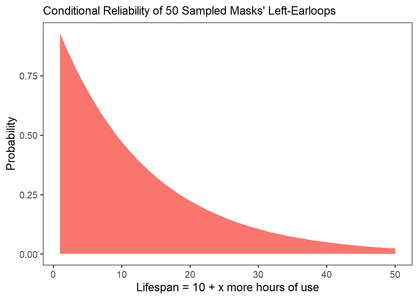
So, what’s the probability that a left-earloop that has lasted 10 hours will last another 5 hours?
## [1] 0.6878039Looks like there’s a 69% chance it will last another 5 hours, given that it has already lasted 10 hours.
Let’s finish up by building ourselves a nice Conditional Reliability function cr, which which calculates the conditional probability of any item surviving x more hours given that it survived t hours and a mean failure rate of lambda.
cr = function(t, x, lambda){
  # We can actually nest functions inside each other,
  # to make them easier to write
  r = function(t, lambda){ exp(-1*t*lambda)}

  # Calculate R(x + t) / R(t)
  output <- r(t = t + x, lambda) / r(t = t, lambda)

  # and return the result!
  return(output)
}## [1] 0.6878039If we were to visualize our conditional reliability function cr below as x ranges from 1 to 50, it would produce the following curve.
19.3.2 \(\mu(t)\): Mean Residual Life
The Conditional Reliability Function \(R(x|t)\) also allows us to calculate the Mean Residual Life (MRL, a.k.a. \(\mu\)) at time \(t\).
The MRL at time \(t\) refers to the average number of years the product is expected to survive after time \(t\). We can calculate it using the distribution below.
\[MRL(t) = \mu(t) = \int_{0}^{\infty}{ R(x|t)dx} = \frac{1}{R(t)} \int_{0}^{\infty}{ R(x) dx} \] It shows the mean expected remaining life years after \(t\).
We can formalize this as function mu(t, lambda). (Since the Greek letter \(\mu\) is pronounced mu.)
# Conditional Reliability
library(mosaicCalc)
library(dplyr)

# Calculate Mean Residual Life
mu = function(t = 5, lambda = 0.001){
  #t = 5
  #lambda = 0.001
  # Get the Reliability Function for exponential distribution
  r = function(t, lambda){ exp(-1*t*lambda)}

  # Get the integral of R(x), the time remaining (mttf)
  integral = antiD(tilde = r(x, lambda) ~ x, lower.bound = 0)

  # Now calculate mu(), the Mean Residual Life function
  # as of time t
  output <- integral(x = Inf, lambda = lambda) * 1 / r(t = t, lambda = lambda)

  return(output)
}
Let’s test it out!
## [1] 1648.721## [1] 7389.056## [1] 148413.2Notice also that when t = 0, we have a mu(0) which equals the MTTF.
## [1] 1000# Get mean time to failure function...
mttf = antiD(tilde = r(t, lambda) ~ t)
mttf(t = Inf, lambda = 0.001)## [1] 1000Works perfectly!
This can also be applied to other life distributions, which we explore in later chapters. For example, here’s a exmaple using the Weibull’s reliability function r(t, m, c).
muw = function(t = 5, m = 2, c = 20000){
  #t = 5; m = 2; c = 20000
  # Get the Reliability Function for exponential distribution
  r = function(t, m, c){ exp(-1*(t/c)^m) }

  # Get the integral of R(x), from 0 to infinity
  integral = antiD(tilde = r(x, m, c) ~ x, lower.bound = 0)

  # Now calculate mu(), the Mean Residual Life function at time t
  output <- integral(x = Inf, m = m, c = c) * 1 / r(t = t, m = m, c= c)

  return(output)
}
# Try it!
# see how this mean residual time to failure gets a little bigger as we move forward?
muw(t = 500, m = 2, c = 20000)
## [1] 17735.62## [1] 17735.66## [1] 17735.71
Learning Check 3
Question
A competing firm produced a mask with a wire that fails at a constant rate of 1 failure per 240 hours.
The probability that the wire survives 1 week (
t = 168hours) in continuous use is… (You buy the mask, and it works without failure for 2 weeks (
t = 336hours) The probability the wire will snap during the next week (t = 504hours) is…
[View Answer!]
- The probability that the wire survives 1 week (
t = 168hours) in continuous use is… (
# Write the reliability function
r = function(t, lambda){ exp(-1*t*lambda)}

# Probability it survives 1 month (760 hours) is...
r(t = 168, lambda = 1 / 240)
## [1] 0.4965853- You buy the mask, and it works without failure for 2 weeks (
t = 336hours) The probability the wire will snap during the next week (t = 504hours) is…
# We can calculate it 2 ways.

# First, we can take
# R(t + x) / R(t)
r(t = 504, lambda = 1 / 240) /
  r(t = 336, lambda = 1 / 240)
## [1] 0.4965853# Or, we can calculate the failure function
f = function(t, lambda){1 - exp(-1*t*lambda)}
# And just calculate the rate of F(t = x)
# Because lambda is a constant failure rate
f(t = 168, lambda = 1 / 240)## [1] 0.5034147
19.4 System Failure with Independent Failure Rates
Consider a mask with a left and right earloop, which have independent failure rates \(\lambda_{left}\) and \(\lambda_{right}\). What’s the probability that the left loop fails before the right loop?
We can express this as:
\[ P(j \ fails \ first) = \frac{ \lambda_{j}}{ \sum_{i=1}^{n}{ \lambda{i}} }\]
In other words, the probability that component \(j\) fails first reflects how big \(\lambda_{j}\) is relative to all the other failure rates in total.
Let’s test this out with our masks dataset.
masks %>%
  summarize(
    # Calculate failure rates of left and right loops
    lambda_left = 1 / mean(left_earloop),
    lambda_right = 1 / mean(right_earloop),
    # Calculate the total probability of either loop failing
    lambda_sum = lambda_left + lambda_right,
    # Calculate probability the left loop fails first
    prob_left_first = lambda_left / lambda_sum)
## # A tibble: 1 × 4
## lambda_left lambda_right lambda_sum prob_left_first
## <dbl> <dbl> <dbl> <dbl>
## 1 0.0749 0.0943 0.169 0.442
19.4.1 Reliability Functions with Multiple Inputs
Suppose a fraction of our masks are shipped in from manufacturer 1, while some are shipped from manufacturer 2. A fraction \(p\) is coming from manufacturer 1, while \(1-p\) is coming from manufacturer 2. We can use the rules of total probability to calculate the reliability function and other quantities for this mask:
\[R(t) = \sum_{i=1}^{n}{ ( \ p_{i} \times R_i(t) \ ) } = \sum_{i=1}^{n}{ ( \ p_{i} \times e^{-\lambda_{i} t} ) }\]
\[MTTF = \sum_{i=1}^{n}{ \frac{p_i}{\lambda_{i}}}\]
\[f(t) = \frac{-d}{dt}R(t) = \sum_{i=1}^{n}{p\lambda_{i}e^{-\lambda_{i}t}}\]
\[z(t) = \frac{ f(t) }{ R(t)} = \frac{ \sum_{i=1}^{n}{p\lambda_{i}e^{-\lambda_{i}t}} }{ \sum_{i=1}^{n}{ ( \ p_{i} \times R_i(t) \ ) } } \]
It’s pretty messy, but powerful!
Suppose we order 75% of our stock from a manufacturer with a failure rate of 1 fabric tear per 50 hours, but 25% from our stock from a manufacturer with a failure rate of 1 tear per 100 hours. What is the (1) overall mean time to failure and (2) overall failure rate at 100 hours for any random mask in your supply?
We can tally this up in a stock data.frame.
To calculate the MTTF, we just take the sum of the fraction of each proportion and each failure rate lambda.
##   mttf
## 1 62.5
To calculate the overall failure rate, we will generate the reliability function, take its derivative to get the PDF.
# Let's write an exponential reliability function
r = function(t, lambda){ exp(-1*t*lambda) }

# Let's derive an exponential PDF f(t), using mosaicCalc's D()
f = D(-1*r(t, lambda) ~ t)
Then, we use the PDFs \(f_i(t)\) and the Reliability functions \(R_i(t)\) to get calculate the overall failure rate \(z(t)\).
stock %>%
  summarize(
    total_f = sum(prob * f(t = 100, lambda = lambda)),
    total_r = sum(prob * r(t = 100, lambda = lambda)),
    z = total_f / total_r)
## total_f total_r z
## 1 0.002949728 0.1934713 0.01524633We could even write it as a function, where p and lambda are equal length vectors for plant 1, plant 2, plant 3, … plant \(n\).
z = function(t){
  # Set the input percentages of products from plants 1 and 2
  p = c(0.75, 0.25)
  # Set the failure rates for each
  lambda = c(0.02, 0.01)


  # Let's write an exponential reliability function
  r = function(t, lambda){ exp(-1*t*lambda) }
  # Let's derive an exponential PDF f(t),
  f = D(-1*r(t, lambda) ~ t)

  # Calculate total probability
  total_f = sum( p * f(t, lambda) )
  # Calculate total reliability
  total_r = sum( p * r(t, lambda) )

  # Calculate overall failure rate
  z = total_f / total_r

  return(z)
}
# Try it out!
z(t = 1)
## [1] 0.0174812## [1] 0.01730786## [1] 0.01524633
19.4.2 Phase-Type Distributions
One way to more accurately model the lifespan of a product is to accept that its failure rate may remain constant, but it might change between failure rates as it passes through phases. Let’s model that!
We can write the time \(T\) to critical failure (via either overstress OR degraded failure) as \(T = min(T_c, T_d+T_{dc})\).
The total probability of a product being in any phase \(a_{i \to n}\) equals 1.
\(a_c = 25\%\)
\(a_d = 40\%\)
\(a_dc = 10\%\)
We can represent it in a dataframe, like so:
myphase <- data.frame(
  id = 1:4,
  phase = c("c", "d", "c", "dc"),
  alpha = c(0.25, 0.40, 0.25, 0.10),
  lambda = c(0.50, 1, 0.50, 3)
)
And, using the same tricks from the preceding section, we can calculate z(t), the overall hazard rate of a phase-type exponential distribution, by taking the sum of the weighted probabilities.
r = function(t, lambda){ exp(-1*t*lambda) }
# Let's derive an exponential PDF f(t),
f = D(-1*r(t, lambda) ~ t)

z = function(t, data){
  output <- data %>%
    summarize(
      prob_f = sum(alpha * f(t = t, lambda)),
      prob_r = sum(alpha * r(t = t, lambda)),
      ratio_z = prob_f / prob_r)
  output$ratio_z %>% return()
}

# Take a peek!
z(t = 1, data = myphase)
## [1] 0.6888965## [1] 0.6161738## [1] 0.5308124## [1] 0.5026807