3 Coding in Python

Welcome to Posit Cloud! You made it! This document will introduce you to how to start coding in Python using Posit Cloud. We will use the Python language frequently to conduct analyses and visualization.

Hello world! We are coding in Python!

Getting Started

Making a Posit Cloud account

We’ll be using Posit Cloud, a browser-based environment you can access from any computer. To get set up, follow your course setup guide, then open the project for this workshop.

Using Python for the First Time

1. For a quick visual orientation, take a peek at the image below.
2. Read and follow along with the instructions on this page. Type the tutorial code and run it in your Python session.

(#fig:graphic_py_1)Visual Intro to Using Posit Cloud

3.1 Introduction to Python

Your project includes a Python script file (its name ends in .py). It contains two kinds of text:

1. code - instructions to our calculator
2. comments - any text that immediately follows a # sign

# For example,
# Comments are ignored by the calculator, so we can write notes.

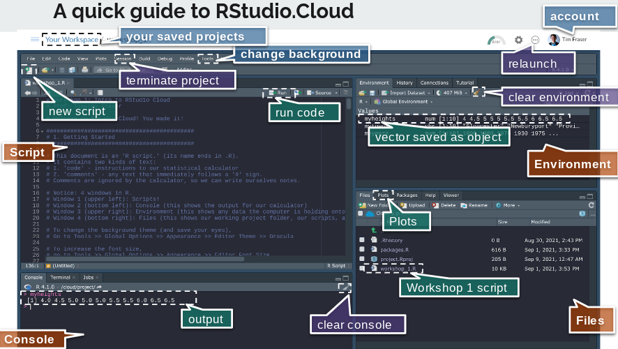
Notice: the IDE has four panes, including the editor, console, environment/history, and files. The console shows outputs from Python (or R).

To create a new script, go to File >> New File >> Text File (or Python Script), then save it and name it.

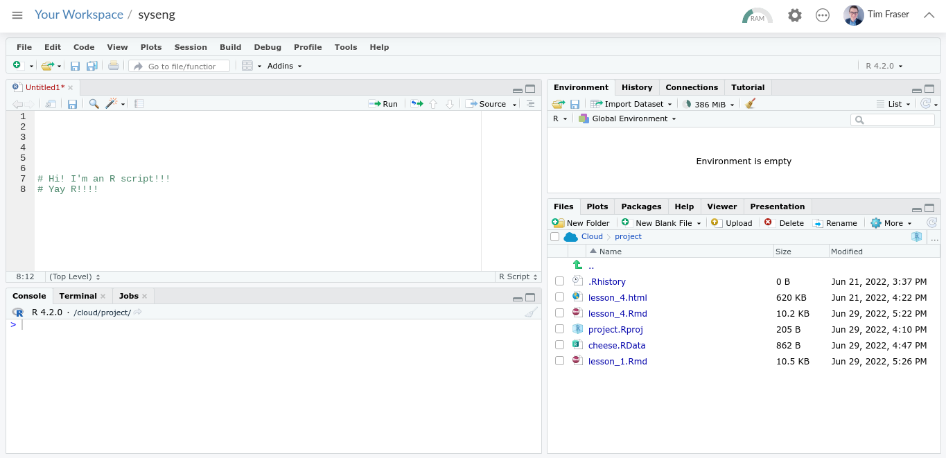
(#fig:image_py_1_1)Open New Script

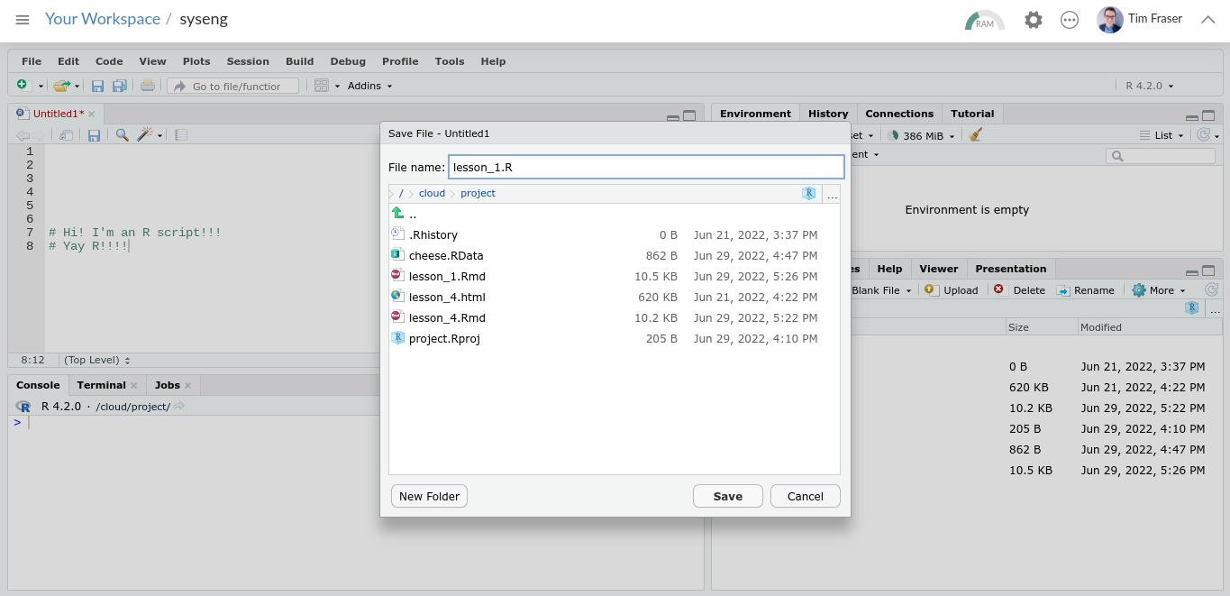
(#fig:image_py_1_2)Save New Script as a .py file!

Let’s learn to use Python!

3.2 Basic Calculations in Python

Try highlighting the following and pressing Ctrl+Enter, or click Run.

Addition:

1 + 5

## 6

Subtraction:

5 - 2

## 3

Multiplication:

2 * 3

## 6

Division:

15 / 5

## 3.0

Exponents:

2 ** 2

## 4

Square roots:

16 ** 0.5

## 4.0

Order of operations still applies. Use parentheses to control order:

2 * 2 - 5

## -1

2 * (2 - 5)

## -6

---

Learning Check 1

Question

Try calculating something wild in Python! Solve for x below using the commands above.

1. \(x = \sqrt{ (\frac{2 - 5}{5})^{4} }\)
2. \(x = (1 - 7)^{2} \times 5 - \sqrt{49}\)
3. \(x = 2^{2} + 2^{2} \times 2^{2} - 2^{2} \div 2^{2}\)

[View Answer!]

((2 - 5) / 5) ** 4

## 0.1296

(( (2 - 5) / 5) ** 4) ** 0.5

## 0.36

(1 - 7) ** 2 * 5 - 49 ** 0.5

## 173.0

2**2 + 2**2 * 2**2 - 2**2 / 2**2

## 19.0

---

3.3 Types of Values in Python

Python commonly uses numeric values and character strings.

15000

## 15000

0.0005

## 0.0005

-8222

## -8222

and

"Coding!"

## 'Coding!'

"Corgis!"

## 'Corgis!'

"Coffee!"

## 'Coffee!'

3.4 Types of Data in Python

3.4.1 Values and Variables

Save a value as a named variable in memory.

2

## 2

"x"

## 'x'

myvalue = 2

myvalue

## 2

Do operations too!

secondvalue = myvalue + 2
secondvalue

## 4

Overwrite variables as needed.

myvalue = "I overwrote it!"
myvalue

## 'I overwrote it!'

Remove variables from memory if needed.

del myvalue
del secondvalue

3.4.2 Lists (like R vectors)

Lists hold multiple values.

[1, 4, 8]

## [1, 4, 8]

and

["Boston", "New York", "Los Angeles"]

## ['Boston', 'New York', 'Los Angeles']

Python will coerce types inside a list only if you mix them when converting to arrays or series. Keep types consistent when possible.

Do math element-wise using pandas Series:

import pandas as p
p.Series([1,2,3,4]) * 2
p.Series([1,2,3,4]) + 2

3.4.3 DataFrames with pandas

Bundle columns into a table using pandas DataFrame.

import pandas as p
myheights = [4, 4.5, 5, 5, 5, 5.5, 5.5, 6, 6.5, 6.5]
mytowns = ["Gloucester", "Newburyport", "Provincetown", 
           "Plymouth", "Marblehead", "Chatham", "Salem", 
           "Ipswich", "Falmouth", "Boston"]
myyears = [1990, 1980, 1970, 1930, 1975, 1975, 1980, 1920, 1995, 2000]

sw = p.DataFrame({
  'height': myheights,
  'town': mytowns,
  'year': myyears
})
sw

Access a column (Series) with dot or bracket notation and do operations.

sw.height
sw.height + 1

Update values as needed.

# sw["height"] = sw["height"] + 1

---

Learning Check 2

Question

How would you make your own DataFrame? Make a DataFrame with 3 columns and 4 rows. Make 1 numeric column and 2 character columns. How many rows are in that DataFrame?

[View Answer!]

import pandas as p
mayhem = p.DataFrame({
  'dogs': ["Mocha", "Domino", "Latte", "Dot"],
  'types': ["corgi", "dalmatian", "corgi", "dalmatian"],
  'treats_per_year': [5000, 3000, 2000, 10000]
})
mayhem

---

3.5 Common Functions in Python

We can compute descriptive statistics using pandas Series methods.

3.5.1 Measures of Central Tendency

sw.height.mean()
sw.height.median()
sw.height.sum()

3.5.2 Measures of Dispersion

sw.height.min()
sw.height.max()
sw.height.quantile(q=0.25)
sw.height.quantile(q=0.75)
sw.height.std()
sw.height.var()

3.5.3 Other Good Functions

len(sw.height)
sw.shape[1]  # number of columns

3.6 Missing Data

Sometimes data include missing values. In pandas these are NaN. Many pandas functions ignore NaN by default.

import pandas as p
mysw = p.Series([4, 4.5, 5, 5, 5, 5.5, 5.5, 6, 6.5, 6.5, None])

mysw.mean()  # returns 5.35, skips None/NaN by default

## np.float64(5.35)

If you need to include missing values in a calculation, convert them or use numpy functions explicitly, but usually skipping them is desired.

---

Learning Check 3

Question

Recreate the table below as a pandas DataFrame named jp, then answer the questions.

town	seawall_m	wave_m
Kuji South	12.0	14.5
Fudai	15.5	18.4
Taro	13.7	16.3
Miyako	8.5	11.8
Yamada	6.6	10.9
Ohtsuchi	6.4	15.1
Tohni	11.8	21.0
Yoshihama	14.3	17.2
Hirota	6.5	18.3
Karakuwa East	6.1	14.4
Onagawa	5.8	18.0
Souma	6.2	14.5
Nakoso	6.2	7.7

1. Reproduce this table as a DataFrame named jp.
2. How much greater was the mean tsunami height than the mean seawall height?
3. Which varied more across towns: seawall height or tsunami height? By how much?

[View Answer!]

import pandas as p
jp = p.DataFrame({
  'town': ["Kuji South", "Fudai", "Taro", "Miyako", "Yamada", "Ohtsuchi", "Tohni", 
           "Yoshihama", "Hirota", "Karakuwa East", "Onagawa", "Souma", "Nakoso"],
  'seawall_m': [12.0, 15.5, 13.7, 8.5, 6.6, 6.4, 11.8, 14.3, 6.5, 6.1, 5.8, 6.2, 6.2],
  'wave_m': [14.5, 18.4, 16.3, 11.8, 10.9, 15.1, 21.0, 17.2, 18.3, 14.4, 18.0, 14.5, 7.7]
})
jp

jp.wave_m.mean()
jp.seawall_m.mean()
jp.wave_m.mean() - jp.seawall_m.mean()

jp.wave_m.std()
jp.seawall_m.std()
jp.wave_m.std() - jp.seawall_m.std()

---

3.7 Packages

3.7.1 Installing packages

Use pip to install packages. Do this once per environment.

%pip install pandas plotnine dfply

3.7.2 Importing packages

import pandas as p
from plotnine import *
from dfply import *

The Pipeline

In Python we can use dfply’s pipeline operator >> to connect data to functions. This reduces parentheses and keeps sequences readable. But it is not as usable as the pipe operator in R. It can only pipe dataframes to common dfply / dplyr functions like select, mutate, summarize, etc.

from dfply import *
sw >> select(X.height)
sw >> mutate(y = X.height ** X.height)
sw >> summarize(mean_value = mean(X.height))

3.8 Visualizing Data with Histograms

We can visualize with matplotlib/pandas, or use plotnine (a Python port of R’s ggplot2) to develope detailed, customized visuals.

3.8.1 pandas/matplotlib

import pandas as p
allsw = p.DataFrame({
  'height': [4, 4.5, 5, 5, 5.5, 5.5, 5.5, 6, 6, 6.5,
             4, 4, 4, 4, 4.5, 4.5, 4.5, 5, 5, 6,
             5.5, 6, 6.5, 6.5, 7, 7, 7, 7.5, 7.5, 8],
  'states': ["MA"]*10 + ["RI"]*10 + ["ME"]*10
})
allsw.height.hist()

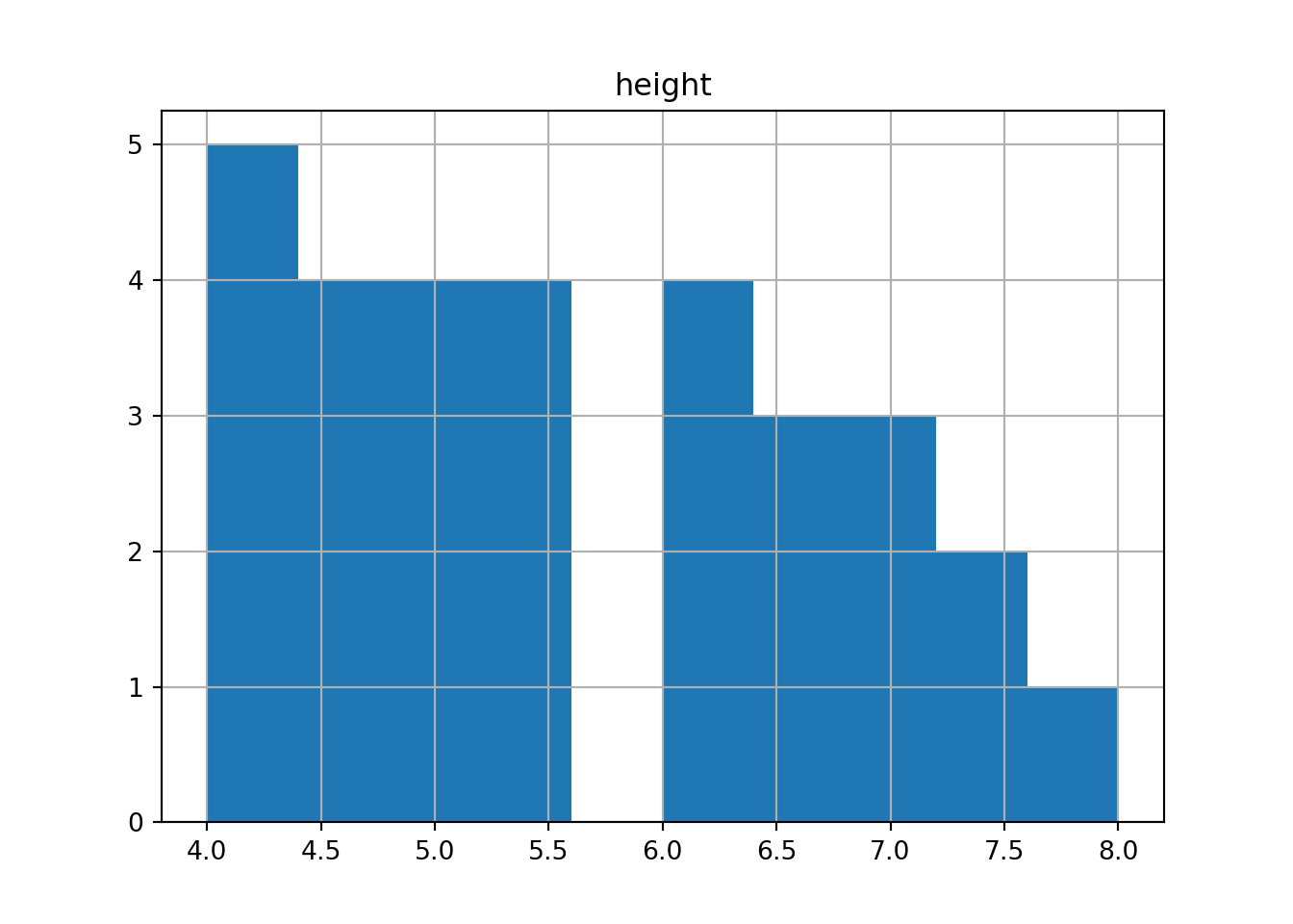
3.8.2 geom_histogram() in plotnine

from plotnine import *
(ggplot(allsw, aes(x='height')) +
 geom_histogram(color="white", fill="steelblue", binwidth=0.5) +
 labs(x="Seawall Height", y="Frequency (# of cities)"))

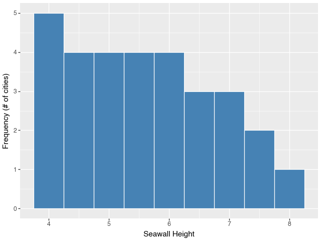
Facet by state:

(ggplot(allsw, aes(x='height')) +
 geom_histogram(color="white", fill="steelblue", binwidth=0.5) +
 labs(x="Seawall Height", y="Frequency (# of cities)") +
 facet_wrap('~states'))

---

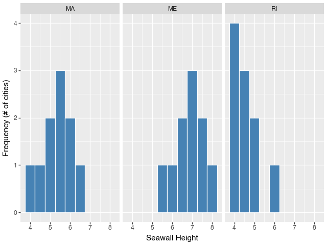
Learning Check 4

Question

Using a list named sw, draw a histogram of the seawall heights: 4.5, 5, 5.5, 5, 5.5, 6.5, 6.5, 6, 5, 4. Use pandas or plotnine.

[View Answer!]

import pandas as p
sw = [4.5, 5, 5.5, 5, 5.5, 6.5, 6.5, 6, 5, 4]
p.Series(sw).hist()

---

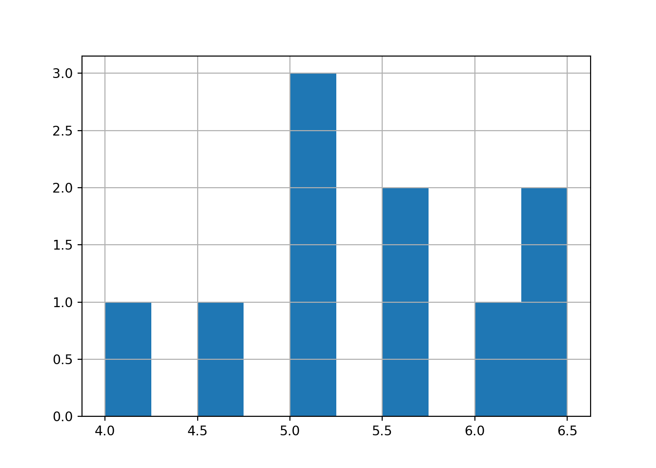
Learning Check 5

Question

Make a histogram of jp['seawall_m'] from Learning Check 3 using (1) pandas and (2) plotnine.

[View Answer!]

jp.seawall_m.hist()

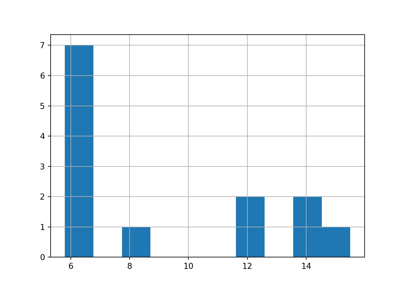
(ggplot(jp, aes(x='seawall_m')) + geom_histogram())

---

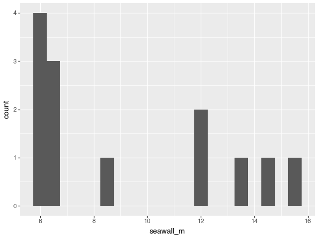
Conclusion

Next Steps

We’ll keep building skills:

• working with data types in Python
• calculating meaningful statistics in Python
• visualizing meaningful trends in Python

Advice

• Clear variables as needed with del or restart the session.
• Clear console outputs and save often.
• Download or upload files from the Files pane as needed.

You’ll be a rockstar at using Python in no time! Stay tuned for our next Workshop!

Troubleshooting

• If your session freezes, use Session >> Restart Session.
• If that doesn’t work, relaunch the project from the top banner menu.
• If that doesn’t work, let me know!